
ความรู้พื้นฐานคณิตศาสตร์ที่จำเป็นในการทำ ตอนที่ 2

วันอาทิตย์ที่, 6 พฤศจิกายน 2565

บันทึกแบบย่อ

จาก pain point ที่สอบแล้วได้คะแนน 7/25
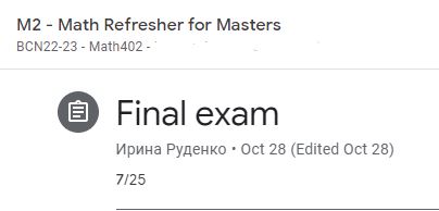
คะแนนสอบคณิตศาสตร์

เลยอยากจะเข้าใจเนื้อหาที่เป็นพื้นฐานของ data science
บทความนี้จึงเป็นการเรียนซ้ำอีกรอบและพื้นฐานแบบย่อตามที่ตัวผมเองเข้าใจ
ดังนั้นแปลว่าอาจจะเข้าใจผิดได้ ถ้าใครเห็นอะไรแปลก ๆ ก็ทักได้เลยนะครับ

และข้อมูลส่วนใหญ่ตัดแปะมาจากในสไลด์ข้อมูลที่ได้เรียนมา
แต่ไม่ได้เอา source มาโดยตรงนะครับเพราะไม่รู้ว่าจะติดลิขสิทธ์ไหม

อีกทั้งการทำสรุปใช้เวลานานมาก เพราะต้องกลับไปเหมือนเรียนใหม่ให้เข้าใจจริง ๆ
ดังนั้นจะค่อย ๆ เพิ่มเติมเนื้อหานะครับ
และหากใครเห็นว่าตรงไหนผมเข้าใจผิดสามารถที่จะบอกได้เลยนะครับ

Linear regression

คือ เรามีข้อมูลหนึ่งชุด แล้วเราก็หาแนวโน้มข้องข้อมูล
โดยเราจะหาตัวแทนเป็นเส้นหนึ่งเส้นที่กลายเป็นตัวแทนของข้อมูลได้

ในและเมื่อเราได้ตัวแทนเส้นเส้นนั้นแล้วเราก็จะประมาณค่าในอนาคตหรือในอดีตได้
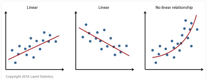
linear regression

ที่มา https://statistics.laerd.com/spss-tutorials/linear-regression-using-spss-statistics.php

5 lines Line 1: Y sub i hat equals b sub 0 plus b sub 1 X sub i Line 2: Y hat sub i equals E s t i m a. t e d o r p r e d i c t e d Y v a. l u e f of o r o b s e r v a. t i o n i Line 3: b sub 0 equals E s t i m a. t e d o f t h of e r e g of r e s s i o n i n t e r c e p t Line 4: b sub 1 equals E s t i m a. t e d o f t h of e r e g of r e s s i o n s l o p e Line 5: X sub i equals V a. l u e o f X f of o r o b s e r v a. t i o n i


6 lines Line 1: Dataset colon the set X comma Y Line 2: X equals the set x sub i sub open brace i equals 1 close brace to the N power comma where x sub i is a. member of r-n features Y equals the set y sub i sub open brace i equals 1 close brace to the N power comma where y sub i is a. member of double struck R Line 3: Model colon Line 4: a. of x equals w sub 0 plus the sum from i equals 1 to n sub features of x sub i times w sub i equals w sub 0 plus x to the T power w Line 5: MSE minimization colon Line 6: Q of open paren a. comma the set X comma Y close paren equals the sum from i equals 1 to N of L of open paren a. of open paren x sub i close paren comma y sub i close paren equals 1 over N the sum from i equals 1 to N of open paren y hat sub i minus y sub i close paren squared right arrow min
2 lines Line 1: Analytical solution colon Line 2: w equals open paren X to the T power X close paren to the negative 1 power times X to the T power Y

● Advantage of Linear regression

- simple and quite effective model when you normalize your data.
  It will be easy to detect which features are important to the model and which are not.

Gradient descent

● Gradient descent method

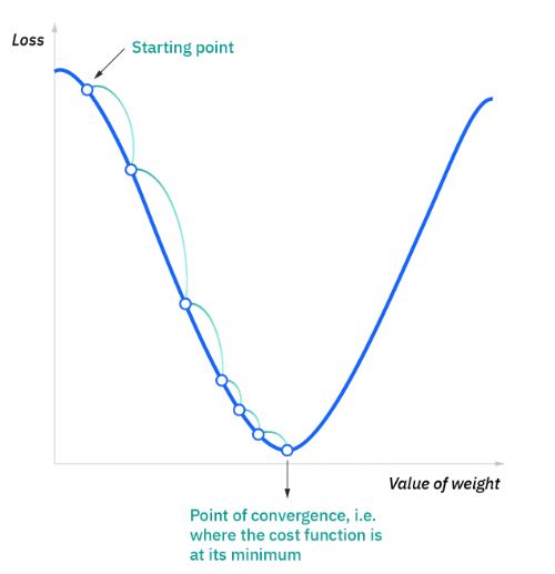
The gradient descent is a numerical optimization method whichallows searching for a local minimum.
2 lines Line 1: bold italic x is a. member of r-n comma f of bold italic x colon r-n right arrow double struck R comma then the gradient is bold nabla bold italic f of bold italic x equals the 3 by 1 column matrix Row 1: the fraction with numerator partial differential f and denominator partial differential x sub 1 times bold italic x Row 2: vertical ellipsis Row 3: the fraction with numerator partial differential f and denominator partial differential x sub n times bold italic x Line 2: Then the gradient descent step is colon bold italic x raised to the n plus 1 power equals bold italic x to the power of n minus gamma nabla f of open paren bold italic x to the power of n close paren comma where gamma is a. member of double struck R is a. constant
gamma open paren g of a. m m a. close paren equals s t e p s i z e
gradient descent 1

ที่มา https://www.ibm.com/cloud/learn/gradient-descent
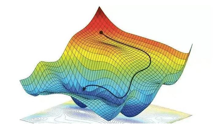
gradient descent 2

ที่มา https://easyai.tech/en/ai-definition/gradient-descent/

Gradient descent is very similar to a rolling ball.

● Gradient descent for linear regression

3 lines Line 1: w to the power of i equals the set w sub 1 to the power of i comma dot dot dot comma w sub n to the power of i minus weights vector Line 2: Q of open paren w comma the set X comma Y close paren minus loss function Line 3: w raised to the n plus 1 power equals w to the power of n minus gamma nabla Q of open paren w to the power of n comma the set X comma Y close paren minus gradient descent step


7 lines Line 1: a. of x equals w sub 1 times bold italic x plus w sub 0 comma bold italic x is a. member of the real numbers Line 2: Q of open paren w comma the set X comma Y close paren equals 1 over N the sum from i equals 1 to N of L sub i of w equals 1 over N the sum from i equals 1 to N of L of open paren a. of open paren x sub i comma w close paren comma y sub i close paren equals 1 over N the sum from i equals 1 to N of open paren a. of open paren x sub i comma w close paren minus y sub i close paren squared equals Line 3: 1 over N the sum from i equals 1 to N of open paren w sub 1 x sub i plus w sub 0 minus y sub i close paren squared Line 4: w raised to the n plus 1 power equals w to the power of n minus gamma nabla Q of open paren w to the power of n close paren minus gradient descent step Line 5: nabla L sub i of w equals nabla open paren w sub 1 times x sub i plus w sub 0 minus y sub i close paren squared equals nabla open paren w sub 1 squared x sub i squared plus w sub 0 squared plus y sub i squared plus 2 w sub 0 w sub 1 x sub i minus 2 w sub 1 x sub i y sub i minus 2 w sub 0 y sub i close paren equals Line 6: open paren 2 w sub 0 plus 2 w sub 1 x sub i minus 2 y sub i comma 2 w sub 1 x sub i squared plus 2 w sub 0 x sub i minus 2 x sub i y sub i close paren Line 7: nabla Q of open paren w to the power of n close paren equals 1 over N sum from i equals 1 to N nabla L sub i of w equals open paren 1 over N the sum from i equals 1 to N of open paren 2 w sub 0 plus 2 w sub 1 x sub i minus 2 y sub i close paren comma 1 over N the sum from i equals 1 to N of open paren 2 w sub 1 x sub i squared plus 2 w sub 0 x sub i minus 2 x sub i y sub i close paren close paren

● Stochastic gradient descent method

Stochastic gradient descent (often abbreviated SGD) is an iterative method for optimizing an objective function with suitable smoothness properties (e.g. differentiable or subdifferentiable). It can be regarded as a stochastic approximation of gradient descent optimization, since it replaces the actual gradient (calculated from the entire data set) by an estimate thereof (calculated from a randomly selected subset of the data). Especially in high-dimensional optimization problems this reduces the very high computational burden, achieving faster iterations in trade for a lower convergence rate. from wikipedia.com

2 lines Line 1: On each step comma choose a. random subset the set X comma Y size l colon the set X to the power of l comma Y to the power of l Line 2: nabla Q of open paren w to the power of n close paren equals 1 over l sum from i equals 1 to l nabla L sub i of w equals open paren 1 over l the sum from i equals 1 to l of open paren 2 w sub 0 plus 2 w sub 1 x sub i minus 2 y sub i close paren comma 1 over l the sum from i equals 1 to l of open paren 2 w sub 1 x sub i squared plus 2 w sub 0 x sub i minus 2 x sub i y sub i close paren close paren

จากตัวอย่างของช่อง StatQuest เขาได้บอกว่าถ้ามี features น้อย ๆ ใช้ในการคำนวน linear gradient descent ก็ไม่เป็นไร
แต่ถ้าหากว่าเราจะคำนวน Genetice feature ที่มี 23,000 ในการทำนายว่าใครจะเป็นเบาหวาน กับประชากร 1,000,000 คน
ถ้าคำนวนแค่ 1,000 step เราจะต้องคำนวน 23,000,000,000,000 ครั้ง ซึ่งมันอึกถึกและทนมาก

ดังนั้นการสุ่มมา 1 ค่า หรือสุ่มมากเป็น batch ที่มากกว่า 1 ค่าจะช่วยลดเวลาและปริมาณในการคำนวนได้เยอะมากประมาณ 3 เท่า

Advantages:
- Speeds up the training considerably
- Allows training on truly big data
- Can be used in a streaming setup when new data arrives over time
Disadvantages:
- May never converge or converge too slowly
- The solution may be unstable

● Choosing the step size is important

Setp size be determined dynamically, affecting the outcome of the optimization.
- When the function value increases after a gradient step, the step-size was too large. Undothe step and decrease the step-size.
- When the function value decreases the step could have been larger. Try to increase the step-size.

Momentum

Momentum optimizationalgorithm (a method of choosing the next weight vector w^(n+1) is defined as follows:

2 lines Line 1: delta w raised to the n plus 1 power equals alpha delta w to the power of n minus gamma nabla Q of open paren w to the power of n close paren Line 2: w raised to the n plus 1 power equals w to the power of n plus delta w raised to the n plus 1 power

which lead to

w raised to the n plus 1 power equals w to the power of n minus gamma nabla Q of open paren w to the power of n close paren plus alpha times open paren w to the power of n minus w raised to the n minus 1 power close paren

Gamma is the learning rate and Alpha is the exponential decay factor determining how much the gradients from the previous steps affect the current step.

ค่า decay rate ที่ดีจะอยู่ที่ประมาณ 0.8-0.9
อันนี้เป็นที่เอามาจาก slide ที่สอน ถามว่าอ่านรู้เรื่องไหม? ตอบว่าไม่ ถถถ

7 lines Line 1: Implementation details Line 2: On iteration t colon Line 3: Compute d W comma d b on the current mini minus batch Line 4: v sub d W equals beta v sub d W plus open paren 1 minus beta close paren times d W Line 5: v sub d b equals beta v sub d b plus open paren 1 minus beta close paren times d b Line 6: W equals W minus alpha v sub d W comma b equals b minus alpha v sub d b Line 7: Line 1: Hyperparameters colon alpha comma beta beta equals 0.9

อันนี้เอามาจากของ Andrew Ng ถามว่ารู้เรื่องไหม ตอบ 20%
เพราะอย่างน้อยก็เห็นว่า beta กับ 1-beta อยู่ด้วยกัน นั่นแปลว่า
ถ้าให้ใส่ค่าน้ำหนักให้ตัวนึกมาก แปลว่าค่าน้ำหนักอีกตัวจะน้อยลงทันที

และลุงเขาให้จินตนาการถึงการกลิ้งบอลลงในถ้วยขนาดใหญ่ เป็นการทำ gredient descent
ถ้าความเร่งของบอลไม่ลดลงเลยบอลก็จะไม่ยอมหยุดนิ่ง
ซึ่งตรงนั้นทำให้บอลไหลข้าม local minimum ไปสู่ global minimum ได้

แต่ที่เข้าใจสุดมากที่สุดมาจากของคุณพี่อินเดียท่านนี้

2 lines Line 1: t sub 1 t sub 2 t sub 3 t sub 4 period period period t sub n Line 2: b sub 1 b sub 2 b sub 3 b sub 4 period period period b sub n a. t t sub n equals b sub n
5 lines Line 1: a. t t equals 1 semicolon V sub 1 equals b sub 1 0 is less than or equal to gamma is less than or equal to 1 w e c h of o o s e gamma equals 0.5 Line 2: V sub 2 equals open bracket gamma times V sub 1 plus b sub 2 close bracket Line 3: equals 0.5 times b sub 1 plus b sub 2 Line 4: V sub 3 equals gamma times V sub 2 plus b sub 3 equals gamma times open paren gamma times V sub 1 plus b sub 2 close paren plus b sub 3 equals gamma squared times b sub 1 plus gamma b sub 2 plus b sub 3 Line 5: i f gamma equals 0.5 semicolon 0.5 squared times b sub 1 plus 0.5 b sub 2 plus b sub 3 equals 0.25 b sub 1 plus 0.5 b sub 2 plus 1 times b sub 3

พี่เขาทำให้เห็นว่าถึงแม้จะเลือก gamma เป็น 0.5
ก็ไม่ได้แปลว่าเราจะสนใจทุกค่าเท่ากัน
แต่เราจะสนใจค่า b ล่าสุดมากที่สุด แล้วสนใจค่า b ก่อนหน้าก็ลดหลั่นตามกันไป

จากที่ไปดูมา momentum ก็จะเร็วกว่า SGD ขึ้นไปอีก

ที่มา https://deepai.org/machine-learning-glossary-and-terms/hyperplane

● Stop criteria

-Small enough (negligible) parameter change

w raised to the n plus 1 power minus w to the power of n is less than epsilon comma where epsilon is greater than 0 and close to 0

-Small enough loss change
-Number of steps limit

● Constrained optimization

ถ้ามีคนให้ function เรามา 1 function แล้วเราจะได้รู้ได้อย่างไรว่าค่าสูงสุดและค่าต่ำสุดของ function นั้นอยู่ที่เท่าไร?
แต่คนที่ให้ function เรามาเขายังแถม constrain หรือข้อจำกัดว่าต้องหาในค่าในช่วงนี้ถึงช่วงนี้เท่านั้นด้วย

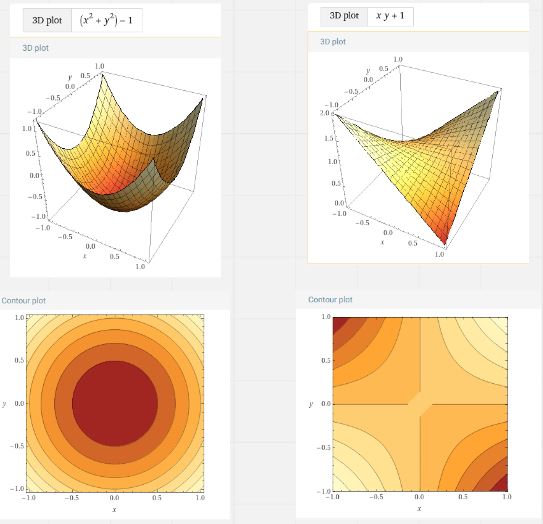
เช่น เขาให้ function f(x) : xy+1 มา
แต่ให้หาค่าสูงสุดและต่ำสุดที่อยู่ในช่วง constrain วงกลมอันนึงมาคือ g(x) : (x^2+y^2)+1
constrain optimization

จากรูปจะเป็น g(x) และ f(x)
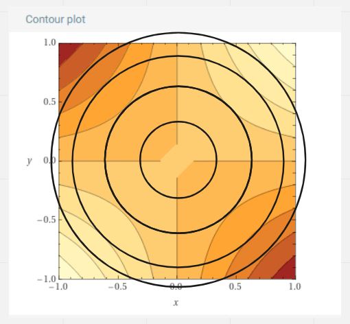
ถ้าเราเอาทั้ง 2 function ที่ได้มาไปฉายลงในกราฟ 2 มิติซ้อนกันเราจะได้หน้าตาประมาณนี้
constrain optimization 2

เราก็จะได้รูปทรงคล้าย ๆ กับถ้วยหนึ่งถ้วยไว้
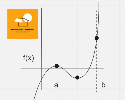
ซึ่งถ้าข้อมูลมันเป็น 2 มิติ เราก็ง่ายหน่อย ในการหา absolute max และ absolute min
โดยเราจะหาได้จากด้านซ้ายสุดหรือขวาสุด

ถ้ากลายเป็น 3 มิติ ค่า domain ของเราก็จะกลายถ้วยและมันก็มีจุดที่เป็นค่าอนันต์
ซึ่งส่วนใหญ่ในชีวิตจริงมิติของข้อมูลจะมีมากกว่า 3
find mimimum and maximum in 2d

Lagrange multipliers

● Lagrange multipliers

script L of open paren x comma lamda close paren equals f of x minus lamda g of x

จากตอนที่ 1 เราจะรู้ว่าจุดสูงสุดและต่ำสุดของ function ค่าความชันจะเป็น 0
แต่ในการใช้ Lagrange เราต้องเขียน constrain ให้อยู่ในรูปของ g(x, y) = k
โดย g=multi-variable function, k=constant

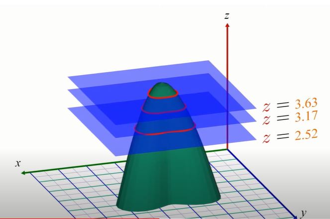
แล้วถ้าเรารูปที่เรา visualize จาก สมการที่ 1 ตอนแรกมาตัดแบ่งตามความสูงของ z ซึ่งเราก็จะได้รูปประมาณด้านล่าง
โดยที่เราจะรู้ค่าความสูงที่จุดไหนเป็นจุดสูงสุด และจุดไหนเป็นจุดต่ำสุดของ function

ถ้าเราค่อย ๆ เลื่อน z สูงขึ้นไปเรื่อย ๆ ไปจุดไหนแล้วไม่ตัดกราฟแปลว่าเราเลยแล้ว
ดังนั้นจุดสุดท้ายที่ยังติดกับกราฟ constrain อยู่นั่นเราจะเดาได้ว่านั่นคือจุดสูงสุด
constrain and levels

ที่มา https://www.youtube.com/watch?v=5A39Ht9Wcu0

ซึ่งเราก็จะเห็นได้ว่าสมการแรกกับสมการที่ 2 จากรูปสีส้มด้านบนหน้าตาไม่เหมือนกัน
แต่การมาตัดสมการที่เป็น g(x) หรือ constrain มันช่วยอะไรเราได้บ้าง?
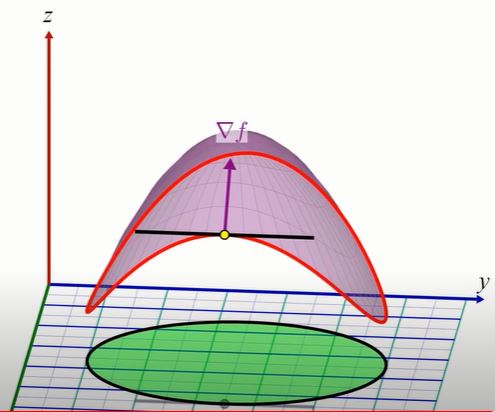
fx pararell gx

ที่มา https://www.youtube.com/watch?v=5A39Ht9Wcu0

ถึงแม้ว่า f(x) และ g(x) แทบจะไม่มีอะไรที่เหมือนกัน
แต่จุดที่ f(x) ตั้งจากกับแกน x เรารู้แน่นอนว่าจุดนั้นมีความชันเป็น 0
ซึ่งแน่นอนว่าหากมันไม่ใช่ "จุดสูงสุด" ก็เป็น "จุดต่ำสุด" อย่างแน่นอน

เช่นเดียวกันกับ g(x) จะต้องตั้งฉากกับแกน x ตรงที่ความชันเป็น 0
ซึ่งเมื่อทั้ง f(x) และ g(x) มีความชันเป็น 0 เหมือนกัน
แปลว่าจุดนั้น f(x) และ g(x) ขนานกัน

ดังนั้นเราจึงได้สมการ Largrange multipliers
ซึ่งตัว multipliers ก็คือค่า lambda แต่นั่นก็ไม่ใช่สาระสำคัญ
เพราะเป็นเพียงตัวบอกว่า f(x) และ g(x) ขนานกันกี่เท่าเฉย ๆ

7 lines Line 1: nabla f equals nabla g Line 2: g equals 0 Line 3: f of open paren x comma y close paren equals x y plus 1 right double arrow nabla f equals left angle bracket y comma x right angle bracket Line 4: g of open paren x comma y close paren equals x squared plus y squared minus 1 right double arrow nabla g equals left angle bracket 2 x comma 2 y right angle bracket Line 5: y equals 2 x Line 6: x equals 2 y Line 7: x squared plus y squared minus 1 equals 0

ทำต่อไปเรื่อย ๆ เราก็จะได้สมการแบบนี้

6 lines Line 1: y equals 2 x Line 2: x equals 2 y Line 3: x squared plus y squared minus 1 equals 0 Line 4: y equals lamda 2 times open paren lamda 2 y close paren equals 4 lamda squared y Line 5: i f y equals 0 comma b o t h s i d e s equals 0 Line 6: else lamda equals plus or minus one half

ในกรณีแรกที่ y = 0 แล้ว x = 0 รูปร่างที่ได้มันไม่ใช่รูปร่างวงกลมที่เราต้องการ
ดังนั้นจึงเหลืออีก 1 กรณีนั่นก็คือ y ไม่ใช่ 0 และเอาค่า lambda ไปแทน
เราก็จะได้ความสัมพันธ์ระหว่าง x และ y

3 lines Line 1: y equals plus or minus x Line 2: s u b t i t u t e i n x squared plus y squared minus 1 equals 0 Line 3: x squared plus open paren negative x close paren squared equals 1 long right arrow x equals plus or minus the fraction with numerator 1 and denominator the square root of 2

และเราก็จะได้จุดมา 4 จุด

2 lines Line 1: max of i m u m equals open paren the fraction with numerator 1 and denominator the square root of 2 comma the fraction with numerator 1 and denominator the square root of 2 close paren comma open paren negative the fraction with numerator 1 and denominator the square root of 2 comma negative the fraction with numerator 1 and denominator the square root of 2 close paren Line 2: min of n i m u m equals open paren the fraction with numerator 1 and denominator the square root of 2 comma negative the fraction with numerator 1 and denominator the square root of 2 close paren comma open paren negative the fraction with numerator 1 and denominator the square root of 2 comma the fraction with numerator 1 and denominator the square root of 2 close paren

ถ้าเราเอาจุด 4 จุดไปแทนในกราฟ จริง ๆ เราก็จะได้จุดสูงสุดและต่ำสุดตามรูป
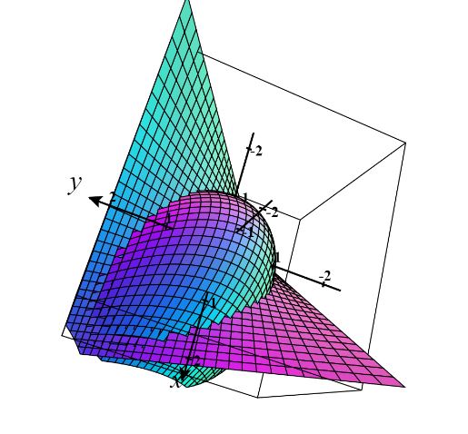
3d plot fx and gx

หรือจะไป plot เล่นเองก็ได้ https://c3d.libretexts.org/CalcPlot3D/index.html

คือจริง ๆ ค่อนข้างเจ็บปวดนะที่ไม่เข้าใจ
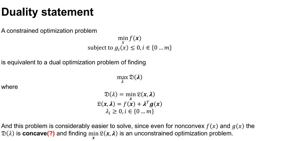
แล้วด้านล่างคือไสลด์ที่เรียนในห้อง บอกเลยว่าอ่านอีก 1,000 รอบก็ไม่เข้าใจ
คือที่ไม่เรียนจากอินเตอร์เน็ตมาคือด้านบนแล้วเอามาสรุป
duality statement

คำว่า duality ทางคณิตศาสตร์หมายถึง
เราสามารถที่จะมองสิ่งใดสิ่งหนึ่งจาก 2 มุมมองได้
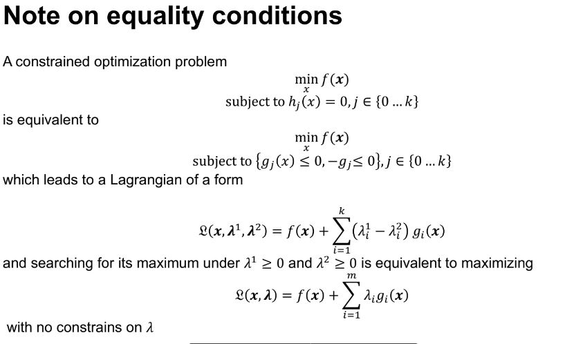
note on equality conditions

ที่เขาเขียนแบบนี้ต้องมีคนเข้าใจแหละ แต่ผมคนนึงที่ไม่เข้าใจ 555
ถ้าเขาเขียนผิดผมก็บอกไม่ได้ว่าผิดตรงไหน 555

● Lagrangian duality in gradient descent

ก่อนที่เราจะเอา lagrangian ไปช่วยในการทำ gradient descent ได้
เราจะต้องรู้อีกเรื่องนึงก็คือ เงื่อนไขของ Karush-kuhn-Tucker ต้องเป็นจริงก่อน

● Karush-Kuhn-Tucker conditions

โดย x optimal ก็ต่อเมื่อมี 3 เงื่อนไขนี้

4 lines Line 1: nabla f of x plus u nabla g of x equals 0 Line 2: g of x is greater than or equal to 0 Line 3: u is greater than or equal to 0 Line 4: u g of x equals 0

เงื่อนไขแรกคือ g(x) >= 0 หมายถึง x ต้องมากกว่าหรือเท่ากับ 0

เงื่อนไขที่สองคือ u >= 0 หมายถึง scalar u ต้องไม่เป็นค่าติดลบ
นั่นแปลว่า f(x) และ g(x) ต้องไม่มี negative coefficients ที่เป็นสัดส่วนกัน
เพราะถ้าเราสามารถที่จะลดค่า g(x) ได้โดยที่ไม่ต้อง optimal ค่า f(x) มันก็ผิดวัตถุประสงค์ของเรา
เพราะเราอยากได้ค่าที่เป็นจุดต่ำสุดหรือจุดสูงสุดของ f(x)

และเงื่อนไขสุดท้าย ug(x)=0 หมายถึง ถ้าสุดท้ายเราเจอค่า x และ u ที่เหมาะสม
มันจะไม่ส่งผลต่อค่า optimal value ในการหาค่า minimization ของเรา
แปลว่า f(x) จะไปวิ่งไปเจอค่าที่ความชันเป็น 0 จริง ๆ

4 lines Line 1: nabla f of x plus u nabla g of x equals 0 Line 2: g of x is greater than or equal to 0 Line 3: u is greater than or equal to 0 Line 4: u g of x equals 0

● Lagrangian duality in gradient descent (ต่อ)

เมื่อทั้ง 3 เงื่อนไขเป็นจริงแล้ว เราค่า Max(lambda >=0) min(x) ของ Lagrangian duality ได้โดย
1) หาค่า x ที่น้อยที่สุดก่อนโดยให้ค่า lambda(u เพราะเอามาจากหลายตำราอาจจะงง ๆ ตัวแปรหน่อย) เป็นค่าคงที่
2) คำนวนหา gradient โดยขยับไปทีละ labmda step
Since L(x, lambda) is concave function f(lambda), this is guaranteed to converge.

บทสรุป

จริง ๆ เรื่อง Lagrangian duality และก็ Karush-Kuhn-Tucker conditions ใช้เวลาเขียนเกือบ 2 วัน
แต่บอกได้เลยว่ายังไม่ได้เข้าใจถึงแก่นจริง ๆ ตอนนี้เข้าใจแค่ concept คร่าว ๆ
แล้วจะตัดจบตอนนี้ไว้ที่นี่เลย แล้วจะได้ขึ้น probability ไว้ตอนใหม่เลย แยกอ่านกันง่าย ๆ
เวลาเลื่อนหาจะได้ไม่ต้องเลื่อนนาน ตอนที่ 3

เขียนโดย กอปกฤษฏิ์ ทรายเขียว

นักเรียนที่ทำสรุปวิชาคณิตศาสตร์ที่เคยได้เรียน

กลับด้านบน