
วันพุธ, 19 ตุลาคม 2565, linear algebra, Matrix, Eigenvector, Eigenvalue, PCA, SVD, calculus, Taylor seires
เนื่องจากเจอปัญในการเรียน Math refresher ตอนปี 2 อย่างมาก
เพราะลืมสิ่งที่เคยเรียนตอนปี 1 แล้ว แม้จะพึ่งผ่านไปไม่นานก็ตาม
อีกทั้งการกลับไปอ่านสรุปในสมุดที่ตัวเองเคยจดที่เคยเข้าใจก็ไม่เข้าใจแล้ว
และสมุดส่วนหนึ่งก็ยุ่ยไปแล้ว(บ่งบอกถึงการดูแลของสมุด 55)
เลยตั้งใจจดให้เรียบร้อยขึ้นและบันทึกลงที่นี่เผื่อเป็นประโยชน์กับคนอื่นด้วยครับ
อีกเหตุผลหนึ่งที่ทำก็เพราะว่า

ดูจากคะแนนสอบครับ 7/25 บอกได้เลยว่าแตกกกก 555
เลยกลับมาทบทวนตัวเองว่าถ้าจะทำงานทางสายนี้จริง ๆ
ไม่ว่าจะอาชีพไหนก็ตามพื้นฐานคือสิ่งสำคัญ และพื้นฐานของ data science คือ math
ดังนั้นผมก็ต้องทำความเข้าใจในสิ่งที่ผมยังไม่เข้าใจ
บทความนี้จึงเป็นการเรียนซ้ำอีกรอบและสรุปคณิตศาสตร์แบบย่อตามที่ตัวผมเองเข้าใจ
ดังนั้นแปลว่าอาจจะเข้าใจผิดได้ ถ้าใครเห็นอะไรแปลก ๆ ก็ทักได้เลยครับ
และข้อมูลส่วนใหญ่ตัดแปะมาจากในสไลด์ข้อมูลที่ได้เรียนมา
แต่ไม่ได้เอา source มาโดยตรงนะครับเพราะไม่รู้ว่าจะติดลิขสิทธ์ไหม
อีกทั้งการทำสรุปใช้เวลานานมาก เพราะต้องกลับไปเหมือนเรียนใหม่ให้เข้าใจจริง ๆ
ดังนั้นจะค่อย ๆ เพิ่มเติมเนื้อหานะครับ
และหากใครเห็นว่าตรงไหนผมเข้าใจผิดสามารถที่จะบอกได้เลยนะครับ
การทำงานของคอมพิวเตอร์ทั้งหมดจะคือการคำนวนกันของตัวเลข
คือการคำนวนกันของชุดข้อมูลที่ถูกเก็บเอาไว้ในรูปของ Matrix และได้ผลลัพธ์เอาไปคำนวนต่อกันไปเรื่อย ๆ
ดังนั้นทุกอย่างที่เราทำในคอมพิวเตอร์ การกดคลิก การเลื่อน scroll แล้วแสดงผลบางอย่าง
ทั้งหมดนี้อยู่ภายใต้การทำงานของ linear algebra ทั้งสิ้น
ยิ่งงานของ data science งานที่ต้องสร้างโมเดลจากข้อมูลโดยตรง
linear algebra จึงเป็นพื้นฐานที่ต้องเข้าใจว่าโมเดลที่เราสร้างมันเกิดขึ้นมาได้อย่างไร
vector = ผลรวมของแรง + ทางทาง ตามระบบ (Cartesian coordinate)
A real-valued vector space (V, +, ⋅ ) is a set of vectors V with two operations
ถ้าเจอเครื่องหมาย < *, * > หมายถึงทำ inner product กัน
A particular type of inner product
ถ้าเจอเครื่องหมาย ( *, * ) หมายถึงทำ dot product กัน
วิธีคิด :
A vector space with inner product is calledan inner product space.
"A finite dimensional real inner product space is called a Euclidean space."
From Introduction to Hilbert Spaces with Applications,
Second Edition by L. Debnath and P. Mikusinski, 1999. Page 92.
ตามที่เข้าใจ norm ก็คือวิธีการวัดระยะอย่างนึง
เนื่องจาก norm เป็นวิธีการวัดอย่างหนึ่ง ดังนั้นแปลว่าเราสามารถวัดค่าหนึ่งได้โดยหลายเครื่องมือ เช่น
คิดง่าย ๆ จับทุกอย่างใส่ในค่าสัมบูรณ์แล้วเอามารวมกัน
L2 จะถือว่าเป็น default norm
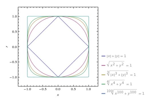
ที่มา https://www.quora.com/What-is-the-mathematical-relationship-between-the-L1-norm-and-L2-norm
เลือกค่าที่ใส่ absolute แล้วมีค่าสูงสุด
Any inner product induces a norm but
case 1 : <x, y> = <y, x>
case 2 : < nx, y> = n<x, y>
case 3 : <x + y, z> = <x, z> + <y, z>
case 4 : if All x > 0 the <x, x> > 0 else <x> == 0
(!) Not every norm is induced by an inner product.
Example : Manhattan norm.
For an inner product vector space, the induced norm satisfies theinequality:
For dot product and Euclidian norm:
The Cauchy-Schwarz inequality says the lengths of the dot product of vectors is less than or equal to the product of the lengths of the vectors.
Another form of this inequality says the length of the sum of two vectors is less than or equal to the sum of the lengths of the vectors.
Distance between two vectors x and y is defined as
For dot product and Euclidian norm, we get Euclidian distance
from Cauchy-Schwarz Inequality
example : angle between x = [10, 0] y =[2, 2]
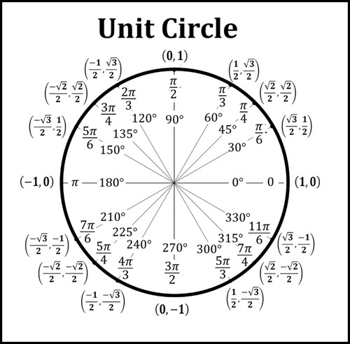
ที่มา https://andymath.com/unit-circle/
x and y are orthogonal if and only if <x, y> = 0.
such as x = [1, 0] and y =[0, 1]
● Orthogonality Projection
Suppose we have two vectors u and v
What is the length of u'v?
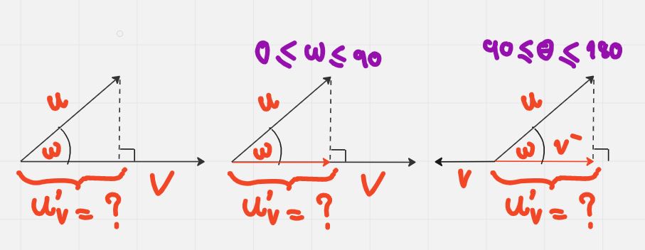
case 1:
case 2:
However
example : u = [ 1, 1, 1] v= [2, 2, 2]
จาก wikipedia
In geometry, a hyperplane is a subspace whose dimension is one less than that of its ambient space. For example, if a space is 3-dimensional then its hyperplanes are the 2-dimensional planes, while if the space is 2-dimensional, its hyperplanes are the 1-dimensional lines.
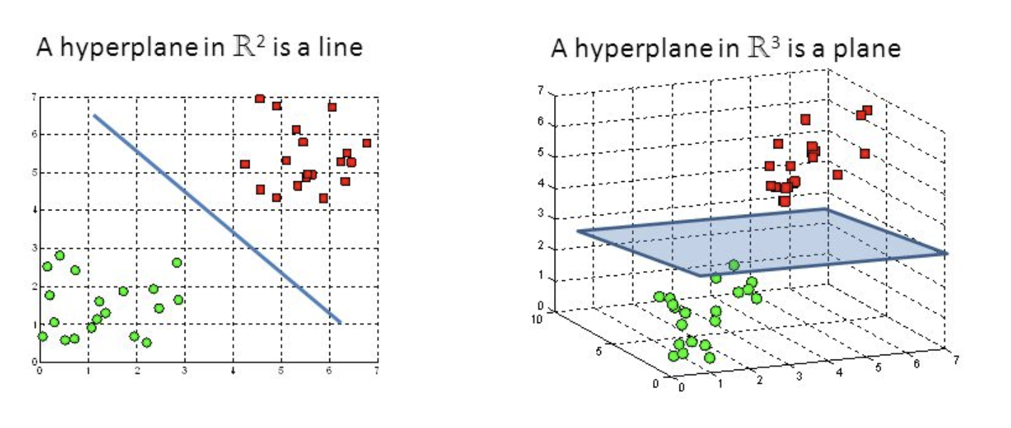
ที่มา https://deepai.org/machine-learning-glossary-and-terms/hyperplane
compact notation:
(w, x) + b = 0, w = (w1, w2, ..., wn) where at least one w ≠ 0
w is a normal vector to this hyperplane
it’s orthogonal to every vector on it.
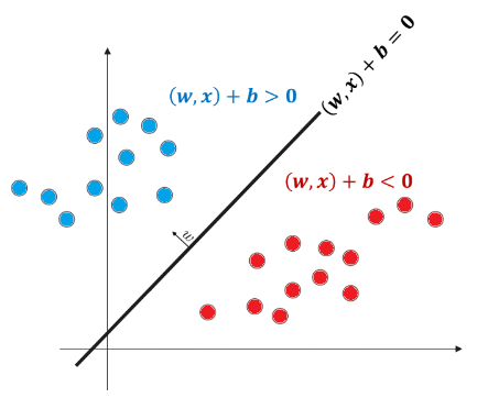
ตรงนี้เป็นตัวอย่างของการใช้ hyperplane ในการทำ binary classification
V = (V, +, ⋅ ) is a vector space
Important thing need to check
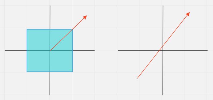
ทั้งสองรูปไม่ใช่ vector subspace ตามคุณสมบัติที่ 2 และ 1 ตามลำดับ
Ploynomail always be Vector subspace :
if degree m <= n and multiply m with a scalar, degree m still <= degree n
vectors can be added together and multipled by scalars.
V - a vector space
A set of all linear combinations of vectors in V is called a span
จากตัวอย่าง span ของ v คืออะไรก็ได้ใน R^3
เพราะเราสามารถจะสร้างอะไรขึ้นมาก็ได้จากการทำ linear combination ของ vector v ที่เรามี
สรุปง่าย ๆ span คือ ผลลัพธ์ที่ได้หลังจากเรา vector ที่มีไปทำ linear combination
คนปรกติจะเขียนในกันรูปนี้ : V = span[v] หรือ V = span[x1, x2, ..., xn] หรือ
Let G be a group, and S a subset of G.
We say that S generates G (and that S is a set of generators for G)
if every element of G can be expressed as a product of elements of S and their inverses.
มีปัญหากับ 2 คำนี้มาก คือ
มีผลเฉลยไม่ชัด (Non-trivial solution) คือ "a[x] = 0 โดยที่ a อย่างน้อย 1 ตัวไม่ใช่ 0"
เช่น u = [1, 2], v=[3, 6]
เราสามารถเขียนได้ในรูป 3v = u
และตรงนี้เป็น linearly dependent
มีผลเฉลยชัด (trivial solution) คือ ต้องเอา a[x] = 0 โดย ทุกตัวของ a = 0
เช่น u = [1, 0], v = [0, 1]
เราต้องแทนค่า a=0 เท่านั้น, au + av = 0
ตรงนี้เป็น linear independent
The linear space V is called n-dimensional
if the maximal number of linearly independent vectors in it is equal to n.
We denote this as dim (V) = n.
- Basis is a set of vectors which can represent every vector in space by linear combination
- A set of n linearly independent vectors e1, e2, ... , en in an n-dimensional space V is called a basis for V.
เช่น x = [1,0,1], y =[1, 1, 1], z =[2, 1, 2]
จะเห็นได้ว่า z = x+y และ x, y linearly independence กัน
ดังนั้น V = span[x, y,z] = span[x,y]
B = {x, y} is a basis of V
orthogonal basis - [e1, e2, ..., en] หรือ basis ของทุกตัวใน v ตั้งฉากกัน
เช่น In R^2 : B = {a1, a2} is a basis of V
a1 = [4, 0], a2 = [0, 3]
orthonormal basis - นอกจาก e ทุกตัวจะตั้งฉากกันแล้ว for all ||ei|| = 1
เช่น In R^3 : : B = {e1, e2} is a basis of V
e1 = [1, 0, 0], e2 =[0, 1, 0], e3 = [0, 0, 1]
จากที่เข้าใจคือ Canonical หมายถึง การตอบให้อยู่ในรูปแบบเดียวที่เป็นพื้นฐาน เช่น
ทำสมการแล้วได้คำตอบ 3/6 อันนี้คือไม่ canonical
แต่ถ้าได้คำตอบเป็น 1/2 อันนี้เป็น canonical
จึงคิดเองว่า canonical น่าจะหมายถึงรูปที่ไม่สามารจะลดได้อีกแล้ว
a Coordinate vector is a representation of a vector as an ordered list of numbers that describes the vector in terms of a particular ordered basis. Coordinates are always specified relative to an ordered basis. (from Wikipedia)
v = a1e1 + a2e2+ ... + anen
coordinates of v = [a1, a2, ... , n]
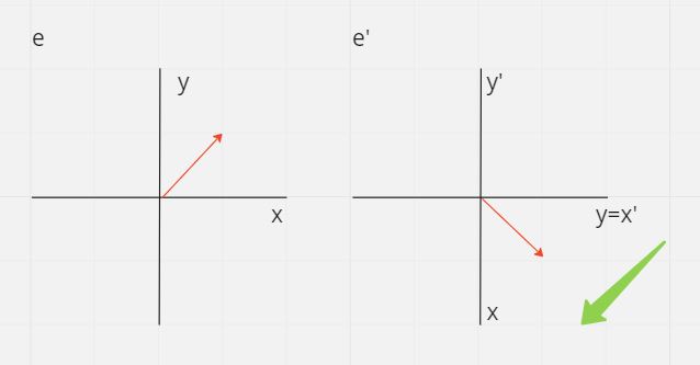
ตามที่เข้าใจคือ สมมติว่าเรามีแกน x และ y แล้วมี vector อันนึงคือ v = [1, 1]
แล้วถ้าเราจับแกนของเราหมุนตามเข็มนาฬิกาไป 90 องศา
ถ้าอยากจะเขียน vector เดิมให้มีทิศทางเดิม เราจะเขียนอย่างไรในแกนใหม่ ที่เป็น x' และ y' ?
เทียบง่าย ๆ คือการใช้คนละแกนเหมือนกับใช้คนละภาษาในการอธิบายสิ่งเดียวกัน
สมมติว่าแกน x' = [0, -1] , y' = [1, 0] แล้ว v เดิม = [1, 1]
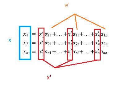
วิธีคิดคือ v[x'] + v[y'] = 1[0, -1] + 1[1, 0] = [1, - 1]
หากเขียนเป็นแถวสวย ๆ จะออกมาแบบนี้ คือ
An n-dimensional vector can be considered nx1 matrix
** An identity matrix may be denoted 1, I, E (the latter being an abbreviation for the German term "Einheitsmatrix"; Courant and Hilbert 1989, p. 7)
Transpose of a Matrix = เปลี่ยนแถวเป็นหลัก เปลี่ยนหลักเป็นแถว
multiplying by scalar
sum of two matrices
multiplying by marix
เอาแต่ละแถวของ A ไปคูณแต่ละหลักของ B
โดยมีเงื่อนไขว่า columns ของ A จะต้องเท่ากับ rows ของ B
ผลลัพธ์ของการคูณกันจะได้ matrix ขนาด rowsA x columnsB
เช่น matrix 2, 6 * martrix 6, 1 = martrix 2, 1
ดังนั้น Vector Space มีคุณสมบัติอะไร Matrix ก็จะมีตามนั้น
การ transformation มีหลายแบบ
แต่การ transform ให้เป็น linear จะต้องมีคุณสมมัติ 2 ข้อคือ
ตรงนี้จะคล้าย กับ change coordinate สามารถย้อนกลับไปอ่านได้
- Every linear transformation can be defined by its matrix.
Columns = how this transformation changes the vectors in the selected basis.
- Vice versa: every square matrix defines some linear transformation.
AxI = A
ดังนั้นการ transform ด้วย identity matrix จะไม่เปลี่ยนแปลงอะไรซักอย่าง
จะเห็นได้ว่าการ project ไปมิติที่ต่ำกว่า จะทำให้ข้อมูลหายไปด้วยบางส่วน
Let A and B be two linear transforms. What if we first apply A and then B?
จากด้านบนถ้า C(x) = D
แล้ว ?(D) = x, แล้ว ? คือ inverse transform
-Not every transform has an inverse!
- Rotation: yes (rotate it back)
- Projection: no เพราะ มิติมันหายไปแล้วบางส่วน
-A matrix that doesn’t have an inverse is called singular. or Determinant(A) = 0
จาก wikipedia.com
In mathematics, the determinant is a scalar value that is a function of the entries of a square matrix. It allows characterizing some properties of the matrix and the linear map represented by the matrix. In particular, the determinant is nonzero if and only if the matrix is invertible and the linear map represented by the matrix is an isomorphism. (a one-to-one correspondence (mapping) between two sets that preserves binary relationships between elements of the sets.)
A numerical way to characterize a linear transformation (and itsmatrix):
- absolute value = how much area changes;
- sign = change of orientation.
สามารถหา Inverser โดยการใช้วิธีการ Gaussian Elimination เทียบกับ Matrix Identity
ถ้าสามารถทำให้ด้านซ้ายกลายเป็น identity ได้
ด้านขวาจะกลายเป็น inverse matrix
The rank of a matrix is the maximum number of its linearly independent rows (or columns).
rank ของ matrix A คือ 2
A set of vectors that are mapped to 0 by a linear transformation A
A*v=0
Vector v is a null space
Ax = b
คำตอบที่ได้จะมีลักษณะดังต่อไปนี้
1. x+y=1, x+y=2 : No solutions, detA=0
2. x+y=1, 2x+y=2 : A single solution x=1, y=0, detA != 0
3. x+y=1, 2x+2y=2 : Infinitely many solutions, b=[1, 2]^T
detA = 0 because A maps onto the same vector
Ax = b
Ax=b has a unique solutions iff rank(A|b) = rank(A) = n
Ax=b has infinitely many solutions iff rank(A|b) = rank(A) < n
Ax=b has no solutions iff rank(A|b) > rank(A)
Ax = 0
let V be a set of solutions:
Factorization : 21 = 3*7
A = L*U
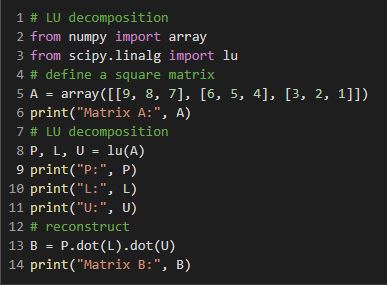
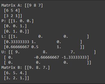
LU code and result
ไว้เข้าใจมากขึ้นจะกลับมาเขียนเรื่องนี้นะครับ เอาแค่ code ไปก่อน 555
The prefix eigen- is adopted from the German word eigen for "proper", "inherent"; "own", "individual", "special"; "specific", "peculiar", or "characteristic".
eigenvector : v = characteristic direction
eigenvalues : lambda = information recovery
eigenvector : v = characteristic direction
eigenvalues : lambda = information recovery
จะเห็นได้ว่า ถ้าหาก det(A-lambdaE) = 0
นั่นแปลว่า matrix(A-lambdaE) ได้ทำการ map ตัวเองไปในมิติที่ต่ำกว่าเดิม
หรือมันคือการลดมิติข้อมูลนั่นเอง
การแยกองค์ประกอบที่สำคัญออกมาทำให้เราได้ basis ที่ดี
ดังนั้นเราจะสามารถเก็บข้อมูลเดิมโดยใช้พื้นที่น้อยลงได้ เพราะเอา basis ที่ดีมาอ้างอิง
และการคำนวนข้อมูลที่น้อยลงแต่มีคุณสมบัติใกล้เคียงกับเดิม
จะช่วยประหยัดทรัพยากรในการคำนวนลงได้อีก
eigenvector จะหมายถึงทิศทางที่เราจะเก็บข้อมูลจากข้อมูลเดิม
เราจะมองจากมุมไหนให้เราเห็นสิ่งนั้นชัดเจนที่สุด และคงคุณสมบัติได้มากที่สุด
อย่างไรก็ตามบางอย่างไม่มี eigenvector เพราะไม่ว่าทางไหนก็เบลอไปหมด ไม่ลักษณะอะไรเด่น
eigenvalues หมายถึงความชัดของเงาที่ได้
โดยยิ่งค่า lambda มาก แปลว่าภาพที่ได้จะยิ่งชัด
the concept of degenerate is "A limiting case in which a class of object changes its nature so as to belong to another, usually simpler, class."
เช่น วงกลมที่ถูกลดพื้นที่จนสุดท้ายกลายเป็นจุด, สี่เหลี่ยมที่ถูกเขียนเป็นสามเหลี่ยมแทน สามเหลี่ยมที่ถูกเขียนให้กลายเป็นเส้นตรง
จะเห็นได้ว่าจาก eigenvector ที่ควรจะเป็น 2 มิติถูกลดให้กลายเป็น 1 มิติแทน
ถ้าเป็น Degenerate Matrix ก็จะทำ Eigen-Decomposition ไม่ได้
Matrix diagonalization is the process of taking a square matrix and converting it into a special type of matrix--a so-called diagonal matrix--that shares the same fundamental properties of the underlying matrix.
ด้านซ้าย คือการทำ Eigendecomposition ส่วนด้านขวาคือ การทำ Diagonalization ถ้าทำด้านซ้ายได้ก็จะทำด้านขวาได้
โดยผลลัพธ์ที่จะได้เป็น diagonal matrix
การทำ Diagonalizable Matrix จะทำให้เราได้ diagonal matrix ที่มีค่าเป็น eigenvalues ของ matrix A
If A is a real symmetric matrix then
1) A has only real (possibly repeating) eigenvalues
2) A has n linearly independent eigenvectors
3) v1, v2, ..., vn are orthogonal or orthonormal
หลายคนคงอาจจะงงมาว่าที่เขียนมายืดยาวเอาไปใช้อะไรได้
โดยปรกติถ้าเราจะเอา Matrix A ไปคูณกัน 8 ครั้ง
สิ่งที่เราต้องทำก็คือ A*A*A*A*A*A*A*A= [A*A]*[A*A]*[A*A]*[A*A] =[A*A*A*A]*[A*A*A*A]=[A*A*A*A*A*A*A*A]
ในทางกลับกันถ้าเราหาเจ้าตัวด้านล่างได้ เราจะสามารถคิดอีกแบบได้นั่นคือ
โดยการทำนวนจะง่ายกว่ามากเพราะว่า ตัวตรงกลางเป็น Diagonal Matrix
ลองคิดง่าย ๆ ว่าถ้าหากเรามีค่า parameter 1 ล้านตัว คูณกัน 1,000 ครั้ง การคูณกันตรง ๆ กับ
การคูณโดยใช้ eigen values basis แบบไหนจะน่าชื่นใจมากกว่ากัน
Orthogonal vectors are linearly independent → A is a fullrank matrix. So, A has an inverse
PCA is an unsupervised learning method that is often reduce the dimensionality of
the dataset by tranform a large dataset into a lower dimensional dataset that
still contain most of the information of the large dataset.
PCA is a powerful statistical tool for analyzingdata based on eigen decomposition.
Suppose we have a dataset with n observations and m features:
Assuming that X is centered, otherwise we should center it firse
because centering matrix will be play an important role.
We will use it to remove the column means from a matrix that each column has mean zero.
how to center matrix
Key idea: project your m×n data onto a p-dimensional subspace (p < m) in such away that we preserve as much variance in our data as possible.
Suppose that this subspace has an orthonormal basis B
How to find B? we should project on the p eigenvectors of the data covariance matrixthat correspond to p largest eigenvalues!
Important to know before do PCA
variance : refers to a statistical measurement of the spread between numbers in a data set.
covariance : Covariance between two random variables = measure of the joint variability.
another thing that we should remember that is eigen decomposition concept
S = Covariance Matrix
another thing that we should remember that is eigen decomposition concept
Why this is useful? because if you have to matirx A is a 1000×2 matrix.
and you have to calculate A*A^T that is 1000*1000 matrix
you should just compute (A^T)*A instead!
-Subtract mean from X
-Calculate Cov(X, X)
-Calculate eigenvectors and eigenvalues of the covariance matrix
-Sort the eigen vector according to their eigenvalues in decreasing order
-Choose first k eigenvectors and that will be the new k dimensions
-Transform the original n-dimensional data points to k dimensions (Project with dot product)
-Only symmetric matrices are guaranteed to have n linearlyindependent eigenvectors (The Spectral Theorem).
-Non-symmetric matrices may or may not have eigenbasis.
-And what about non-square matrices?
Singular Value Decomposition is a generalization of eigen decomposition for all matrices.
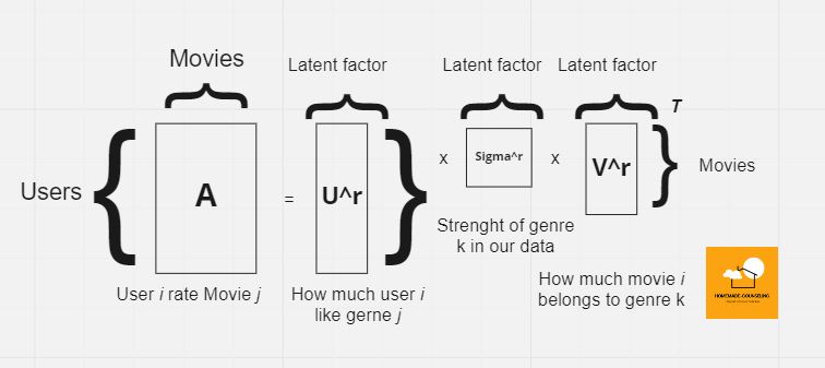
สมมติว่าเรามีข้อมูลขนาด 1 ล้าน * 1 แสน
การคูณ matrix ขนาด n*n เราจะต้องคูณกัน n^3 ครั้ง
เช่น matrix 2*3 เราจะต้องคูณกันทั้งหมด 8 ครั้ง
การที่เราจะเอาทั้งหมดมาคำนวนกัน RAM ของพิวเตอร์ของเราไม่ไหวแน่นอน
ดังนั้น เราก็แบ่งมันเป็นย่อย ๆ แล้วค่อย ๆ คิดได้
และคิดด้วยเลขที่มี 0 เยอะ ๆ คอมก็จะทำงานได้เร็วขึ้นมาก
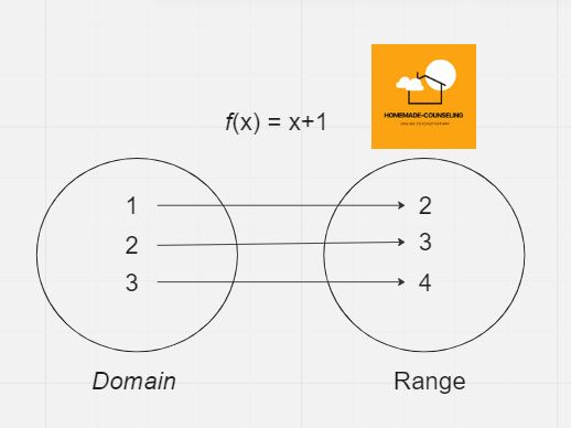
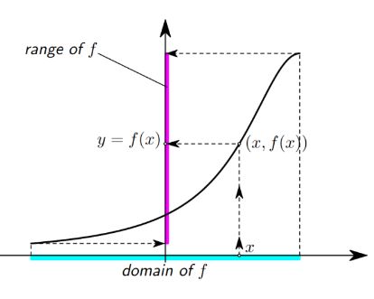
Function describes the relationshipbetween x and y.
-Domain: the set of numbers for which a function is defined. ,สิ่งที่เอาไปใส่ใน f(*)
-Range: the set of all possiblenumbers f(x) as y runs over itsdomain. ,ผลลัพธ์ที่ได้จากการเอา f(*)
univariate = มีตัวแปรเพียงตัวเดียวในการพิจารณา
bivariate = มีตัวแปรสองตัวในการพิจารณา
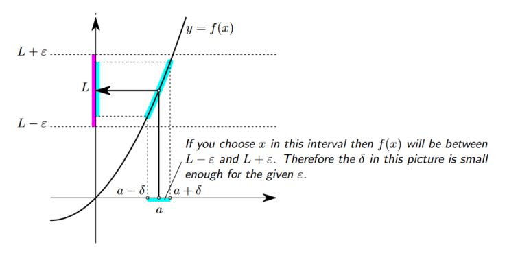
-“The limit of f(x) as x approaches a is L”.
-Informally: for x close to a, f(x) is close to L. The closer x gets to a, the closer f(x) gets to L.
แปลเป็นภาษามนุษย์จะมีความหมายประมาณนี้ครับ
- continuous function : a function that can be drawn in one stroke.
example of discontinuous function
f(x) = 1/x
-increaseing funcstion : y=f(x)
-decreaseing funcstion : y=f(x)
monotonic function is a (non-) increasing / decreasing function over the whole domain.
there are a monotonically non-decreasingfunction, a monotonically non-increasing function
and a non-monotonic function.
Derivative is way to measure change
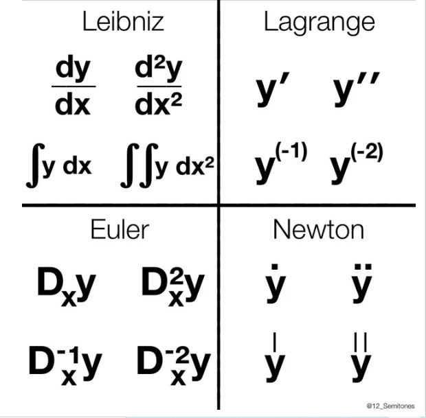
คือแต่ละคนคิดก็ใช้สัญญะไม่เหมือนกัน พอคนมาเรียนก็เลยงง
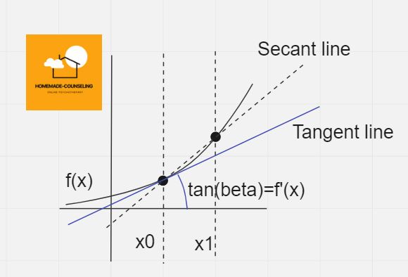
แต่จริง ๆ แก่นแท้ของมันคือการเปรียบอัตราการเปลี่ยนแปลงระหว่างจุด 2 จุด
Geometrically, the derivative of a function f(x) at a given point is the slope of the tangent to f(x) at the point a.
สมมติว่าเรามีหนึ่งฟังชั่น คือ f(x) = x^3-12x+2
เรารู้ว่าที่ที่ความชันเป็น 0 จะเป็นจุดสูงสุดหรือต่ำสุด เราจะเรียกจุดนี้ว่า Critical Point
f'(x)= 3x^2-12 หากเราแก้สมการนี้โดยการเท่ากับ 0 : 3x^2-12=0
เราจะได้ค่า x มาสองค่าคือ 2 และ -2
หรือ f'(2)=0 และ f'(-2)=0
จากรูปจะเห็นได้ว่าที่จุด x=-2 ค่า derivative ที่จะได้จะข้ามจากค่า + ไปเป็นค่า -
เป็นเกณฑ์วัดว่านั้นคือจุดสูงสุด
และที่จุด x=2 ค่า derivative ที่จะได้จะข้ามจากค่า - ไปเป็นค่า +
เป็นเกณฑ์วัดว่านั้นคือจุดต่ำสุด
สามารถย้อนไปดูรปก่อน ๆ ที่เป็นค่า tangent ได้ครับ
หากเราดูที่กราฟด้านล่างที่อยู่ในช่วงของ [a, b]
เราจะเห็นได้ว่ามีจุดที่สำคัญอยู่ 3 จุด ไล่จากซ้ายไปขวาคือ
1) local maximum
2) the minimum for the region under cosideration
3) the maximum for the region under cosideration
ดังนั้น Don’t Forget the Endpoints of the interval!
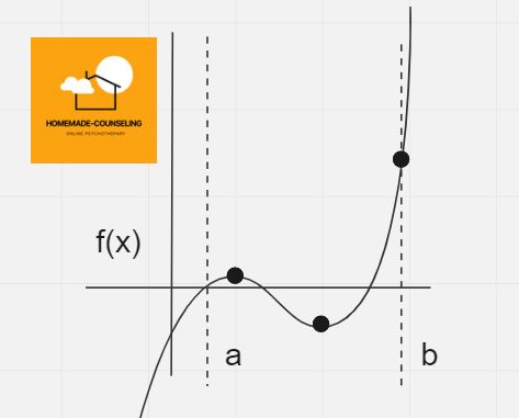
Suppose you need to find global maxima (minima) of f(x) on [a, b]
Step :
1) Find all critical points of f(x) on [a, b]
2) Determine which of them are the local maxima (minima);
3) Compute f(x) at the endpoints: f(a) and f(b) .
4) Pick the point from (2) – (3) corresponding to the largest (smallest) functionvalue.
Derivatives of the derivatives looks like this
f''(x)=(f'(x))', f'''(x)=(f(f''(x))', ...
Let a be a stationary point: f'(x)=0
as we know from above
if f'(x) < 0 then f(x) has a local maximum at x
if f'(x) > 0 then f(x) has a local minimum at x
However if x = 0 we don't know what happens so we need to check manually
Derivatives of the derivatives looks like this
f''(x)=(f'(x))', f'''(x)=(f(f''(x))', ...
Let a be a stationary point: f'(x)=0
as we know from above
if f'(x) < 0 then f(x) has a local maximum at x
if f'(x) > 0 then f(x) has a local minimum at x
However if x = 0 we don't know what happens so we need to check manually
There are 3 cases that can be possible.
Taylor series are an incredibly important tool for numerical approximation.
The formula for the Taylor series of a function f(x) around a point x=a is given by
Taylor Series เป็นเรื่องนึงที่ผมรู้สึกว่าไม่ค่อยเข้าใจว่าเรียนไปทำไม
แต่ที่ไปหาข้อมูลเพิ่มเติมมาคลิปของ 3Blue1Brown Taylor series | Chapter 11, Essence of calculus
ช่วยผมเยอะมากครับ (จริง ๆ หลายเรื่องที่เข้าใจก็เพราะ 3Blue1Brown 555) และก็เอามากจาก cambridgecoaching
เข้าเรื่องเลย คือ การทำ function ที่เรามีให้อยู่ในรูปของ polynomial มันมีข้อดีหลายอย่างต่อการคำนวน
เอาไปหาก derivative หรือเอาไป integral ได้ทำได้ง่ายอีกเช่นกัน
ยกตัวอย่างเรามี function ที่ค่อนข้างซับซ้อน เช่น f(x) = cos(x)
แล้วเราต้องการสร้าง function ที่ประมาณค่ามีความใกล้เขียนกับ function cos(x) มากที่สุด
เริ่มจากวิธีที่ง่ายที่สุดคือ การสร้าง function เส้นตรง
นั่นคือ g(x) = mx+b และ f(0) = g(0)
เรารู้ว่าค่า cos(0) = 1 เราจะได้สมการ g(0)=m(0)+b=1 ดังนั้นเราจะรู้ว่า b=1
ซึ่งเราจะได้เส้นตรงสีฟ้าแนวนอนขนานแกน x ตามรูปด้านล่าง
แต่เราอยากได้ function ประมาณค่าที่มันใกล้เคียงมากกว่า function เส้นตรง
เราเลยจะสร้าง quadratic funtion ขึ้นมา
ซึ่งหน้าตาของ function ก็จะเป็นประมาณนี้ g(x) = a + bx + cx^2
แต่เราจะได้ สมการมากมายที่ g(0) = 1 + bx+cx^2 ซึ่ง bx+cx^2 = 0 จะทำให้สมการเป็นจริง
ตอนนี้ได้ค่า a = 1 แล้ว
ดังนั้นเราก็จะได้ค่ามากมายที่เอาไปแทนค่าใน b, c และทำให้สามาการเป็นจริง
ไปดูที่พาราโบล่าด้านล่างที่ผ่านจุด (0, 1) แต่อันสีฟ้าเพียงอันเดียวที่ดูแล้วจะใกล้เคียง cos(x) มากที่สุด
โดยเราจะหา g(x) สีฟ้าได้โดย หา derivative ของ g'(x) = f'(x)
สิ่งที่ควรรู้เพิ่มเติม ก่อนไปต่อ
first derivative = slope of the tangent lineto the function at the point x
the first derivative tells us how whethera function is increasing or decreasing,
and by how much it is increasing or decreasing.
second derivative = tells us if the first derivative is increasing or decreasing. If the second derivative is positive, then the firstderivative is increasing, so that the slope of the tangent line to the function is increasing as x increases. We see this phenomenon graphically as the curve of the graph being concave up, that is, shaped like a parabola open upward. Likewise, if the second derivative is negative, then the first derivative is decreasing, so thatthe slope of the tangent line to the function is decreasing as x increases. Graphically, we see this as the curve of the graph being concave down, that is, shaped like a parabola open downward. At the points where thesecond derivative is zero, we do not learn anything about the shape of the graph: it may be concave up orconcave down, or it may be changing from concave up to concave down or changing from concave down toconcave up
เพราะเรารู้ว่าความชันของ f(0) = 0 เพราะเป็นจุดสูงสุด
ที่จุด g'(x) = f'(x) ความชันของ g'(x) และ f'(x) จะต้องเท่ากัน
cox'(0) = -sin(0) = 0
เราก็จะได้ค่า b = 0
และเราก็อยากที่จะได้ค่า c ต่อ โดยเราก็หาโดยการหา second derivative ของ g''(x) = 2c
derivative of f(x) = cos(x) at x=0 is f''(0) = -cos(0) = -1, this gives us that 2c=-1, and so c = -1/2.
เราก็จะได้ค่า c = -1/2
จุดท้ายเราก็จะได้ quadratic approximation แบบนี้
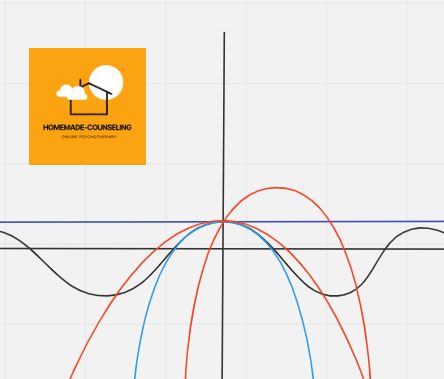
เราก็จะได้ function กำลังสองสีฟ้าที่ดีกว่า function กำลังสองอันอื่น ๆ
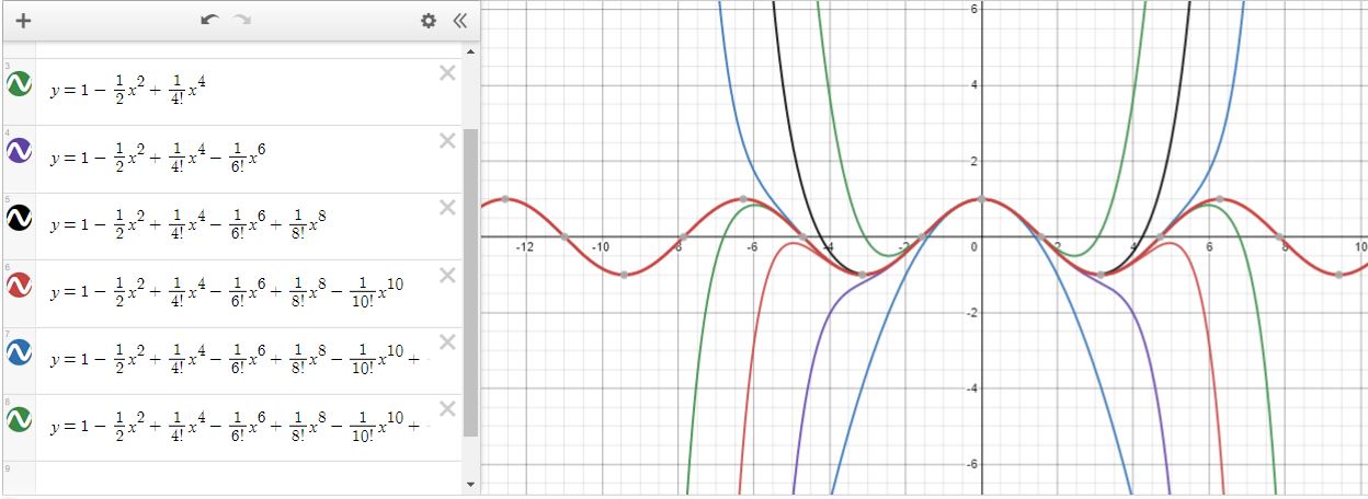
อย่างไรก็ตาม หากเราต้องการ functions ที่ใกล้เคียงมากกว่ากำลังสอง
สิ่งที่เราจะทำก็คือ หา derivative ของ กำลังนั้นลึกลงไปเรื่อย ๆ
f'''(x)=g'''(x) แบบนี้ไปไปเรื่อย ๆ
แล้วเราก็จะได้อะไรแบบนี้
ตอนนี้เริ่มรู้สึกว่าเนื้อหาเยอะเกินไปในบทความเดียว
ดังนั้นผมจะรอเขียนแยกอีกหนึ่งบทความนะครับ ความรู้พื้นฐานคณิตศาสตร์ที่จำเป็นในการทำ AI ตอนที่ 2
ตอนแรกตั้งใจว่าจะตัดแปะเฉย ๆ แปปเดียวก็น่าจะเสร็จ
แต่พอเขียนจริงต้องทำความเข้าใจพร้อมกันไปด้วยอีกรอบในส่วนที่ไม่เข้าใจ
เพื่อตัวเองในอนาคตกลับมาอ่านจะได้อ่านง่าย ๆ ตอนต้องใช้ในอนาคต
พอเขียนจริงเริ่มเขียนตั้งแต่ 19 ตุลาคม 2022 แต่เขียนตอนแรกเสร็จตอน 6 พฤศจิกายน
ใช้เวลาไป 20 กว่าวัน เยอะกว่าที่คิดไว้ตอนแรกมากครับ
แล้วจะค่อย ๆ เขียนเพิ่มเนื้อหาในตอนที่ 2 เพิ่มนะครับ
นักเรียนที่ทำสรุปวิชาคณิตศาสตร์ที่เคยได้เรียน