ความรู้พื้นฐานคณิตศาสตร์ที่จำเป็นในการทำ ตอนที่ 3
ความน่าจะเป็นและสถิติ

วันอาทิตย์ที่, 8 พฤศจิกายน 2565‍

ที่มาของการสรุปสถิติ

เนื่องจากอยากจะเข้าใจเนื้อหาที่เป็นพื้นฐานของ data science
บทความนี้จึงเป็นการเรียนซ้ำอีกรอบและพื้นฐานแบบย่อตามที่ตัวผมเองเข้าใจ
ดังนั้นแปลว่าอาจจะเข้าใจผิดได้ ถ้าใครเห็นอะไรแปลก ๆ ก็ทักได้เลยนะครับ
และข้อมูลส่วนใหญ่ตัดแปะมาจากในสไลด์ข้อมูลที่ได้เรียนมา และหาเพิ่มตามอินเตอร์เน็ต
‍แต่ไม่ได้เอา source มาโดยตรงนะครับเพราะไม่รู้ว่าจะติดลิขสิทธ์ไหม
และไม่กี่อาทิตย์ที่ผ่านมาก็ได้ความช่วยเหลือจาก ChatGPT นิดหน่อยครับ
‍เพราะบางเรื่องผมก็ไม่เข้าใจอยู่ดีต้องไปหาอ่านเพิ่มเอาเอง
‍
อีกทั้งการทำสรุปใช้เวลานานมาก เพราะต้องกลับไปเหมือนเรียนใหม่ให้เข้าใจจริง ๆ
ดังนั้นจะค่อย ๆ เพิ่มเติมเนื้อหานะครับ
และหากใครเห็นว่าตรงไหนผมเข้าใจผิดสามารถที่จะบอกได้เลยนะครับ

จริง ๆ ก็ไม่ค่อยอยากทำแล้วเพราะมันใช้เวลานานมาก แต่รู้ว่ามันต้องใช้จริง ๆ
แล้วก็ไป search หาตรง ๆ มันก็ไม่ค่อยมีคนสรุปสั้น ๆ ให้ในภาษาที่ลิงเข้าใจ
คือคนอื่นเขาเขียนดีกว่าเรานะ แต่เราอ่านไม่เข้าใจไงต้องเสียเวลาทำความเข้าใจนานมาก ถถถ

Probability theory

The subject matter of probability theory is the mathematical analysis of random events, i.e., of
those empirical phenomena which under certain circumstance can by describe by saying that:
1) They do not have deterministic regularity - observations of them do not yield the same outcome
2) They posses some statistical regularity - indicated by the statistical stability of they frequency

Probabilistic Model of an Experiment with
a Finite Number of Outcomes

● Sample Spaces (the space of elementary events)

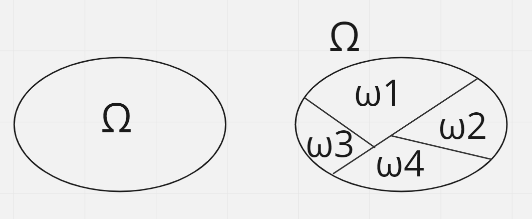
ω แต่ละตัว disjoint กันแล้วเส้นที่แบ่งคือ partition

จะใช้สัญญะลักษณ์โอเมก้าใหญ่(เป็นอักษรตัวสุดท้ายของกรีก) เป็นตัวแทนของ sample space
แล้วใช้ตัวโอเมก้าเล็กเป็นผลลัพธ์ของแต่ละเหตุการณ์ที่เกิดขึ้น

Definition The sample space S of an experiment is the set of all possible outcomes of the experiment.
An event A is a subset ofthe sample space S, and we say that A occurred if the actual outcome is in A.

Example : For a single of toss coin the sample space

● disjoint or mutually exclusive (⊔)

● partition

Partition of Omega is sum sequence of disjoint set that equal to Omega

● indicator function

indicator function of A means we focus only on the event that occurred in A

● De Morgans law

The complement of the union of two sets is the intersection of their complements and the complement of the intersection of two sets is the union of their complements.

For n tosses of a coin the sample space (ordered) is and [unordered] is

● Sampling with replacement and Sampling without replacement

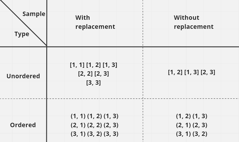
ordered samples = distinguishable objects
unordered samples = indistinguishable objects

● Classic model of distributions or Naive definition of probability

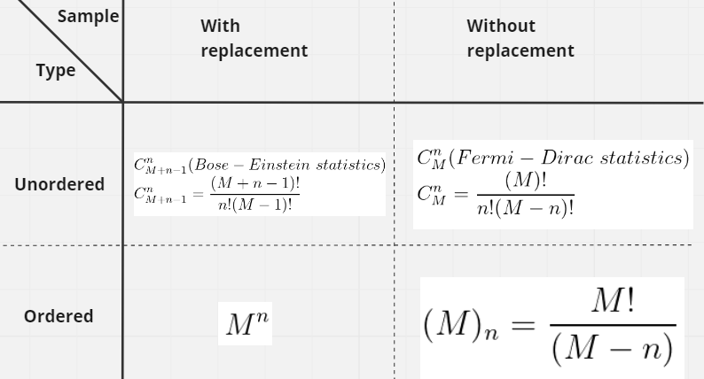
Classical model were based on the belief that any experiment that any experiment can be descriebed in terms that referred to as elementary outcomes of experiment, with the aggregate of all elementary

● Events (A)

The outcome belongs to some subset of the set off all possible outcomes or favorable outcomes.
Some book may use |A| denotes to all number of elements in A.

● probability of the outcome

● Continuity of Probabilities

from what I understand we can think the same way as a normal probability such as sum of all disjoint sets of probability will become the Omega.

● Independent Events

This concept distinguishes probability theory from general theory of measure spaces.

When the change of event A does not affect event B. So event A and B are independent.
‍
Two events A, B are independent to each other if P(AB)=P(A)P(B)
and we can also write that A disjoint B (A⊔B)

Another example for independent

more detail in https://github.com/tutalae/Homemade-Counseling/blob/main/simple_independent_simulation.ipynb

In conclusion, it is possible that each sub-events are dependent on each other.
But finally all events are independent.
Therefore, simple reasoning is not something that should be used to obtain dependency or independency.

● Conditional probability

The probability that event A will happen if event B already happens.

More properties of conditional probability:

Remember that in general P(A|B) ≠P(B|A)
A and B are independent if and only if P(A|B) = P(A)

● A medical test for a disease

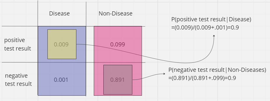
conditional probability of people who get disease and got the positive test result = 0.9
conditional probability of people who not disease and got the negative test result = 0.9
The results of the test kit seem to have an accuracy of .9 or 90%.

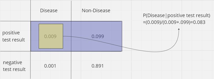
In the case, when you get a positive test result the probability that you will get a disease is only 0.083 or 8.3%
So, don't trust your intuition!

● Bayes' Theorem

It's an important concept in machine learning and ai.

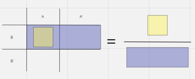
We can calculate the likelihood of A occurring given B has already occurred using the Bayes theorem.
A is the hypothesis and B is the supporting evidence. The predictors and features are assumed to be independent in this situation. In other words, the presence of one feature does not change the behavior of another.
Consequently, it is referred to as naive.

จุดอ่อนของ Baye คือ การคิดค่าความน่าจะเป็นโดยการเอามาคูณกันตรง ๆ
ดังนั้นแล้ว P(A)P(B) =P(B)P(A)
แต่ในบางกรณีแล้ว หากมีลำดับเข้ามาเกี่ยวข้องเช่น การวิเคราะห์ว่า email ไหนเป็น spam
ที่ส่งมาโดยเจ้าชายบรูไนหรืออีออนมัสที่อยากได้ทรูมันนี่
1) ฉัน หิว ข้าว
2) ข้าว ฉัน หิว
ถ้าเป็นคนไทยก็จะรู้ว่าประโยคไหนเป็นประโยคที่ scammer ต่างชาติใส่ google translate มา
แต่หากคิดว่า Baye จะได้ค่าความน่าจะเป็นเท่ากันเพราะเป็นการคำนวนโดยไม่สนใจลำดับ

● Random Variables

Random Variables is any numerical function that define on sample space mapping to outcome to real number

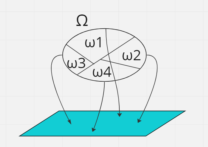
ในที่นี้ X = random variable, รูปเป็นการ map sample space กับ vector 2 มิติ

ยกตัวอย่างการโยนเหรียญ 2 ครั้ง
หากได้หัว(H) เราจะให้ค่า = 1, แต่ถ้าได้ก้อย(T) เราจะให้ค่า = 0
ผลลัพธ์การโยนเหรียญที่ได้จะมี 4 กรณีคือ HH = 2 , HT = 1, TH = 1, TT = 0
ω = HH, HT, TH, TT
ξ(ω) = 2, 1, 1, 0

สมมติ
ω = HHHH แล้ว ξ(ω) = 4
ω = HHHHTH แล้ว ξ(ω) = 5
ω = HHHHTHTH แล้ว ξ(ω) = 6
สรุปอีกครั้งมันคือเอาผลลัพธ์ที่ได้ไม่ว่าจะเป็นอะไรก็ตามไป map กับจำนวนจริง!

ตอนแรกพยายามทำความเข้าใจอยู่นานว่าทำไมถึงใช้ ξ(ω) เพราะถ้าเรามอง เป็น function แล้ว
เพราะถ้าเรามอง เป็น function แล้ว เราสามารถเปลี่ยน ξ เป็น function อื่นได้ เช่น α(ω) β(ω)
หรือ X(ω) จากรูปตัวอย่างด้านบนก็ได้ (อ่านมาหลาย ๆ ที่เขาจะใช้ X แทน)

ถ้าเรารู้ว่า function ที่ใช้คืออะไร เราก็จะรู้ว่าข้อมูลชุดนั้นถูกแจกแจงภายใต้ function นั้น
แล้วเราก็จะรู้คุณสมบัติของการแจกแจงชนิดนั้น ๆ แล้วเอาคุณสมบัติที่เรารู้ว่าใช้ประโยชน์ได้

● Distribution Functions and Probability Functions

ปัญหาเกิดขึ้นเพราะว่า สมมติว่าเราโยนทีละ 2 ครั้งติดกัน เรารู้ว่าผลลัพธ์ที่ได้มีโอกาสออกมาแค่ 4 อย่าง
คือ HH, HT, TH, TT
และเราสามารถวิเคราะห์ความน่าจะเป็นของแต่ละเหตุการณ์ได้โดยสามารถคิดมือได้
แต่ถ้าเราอยากรู้ว่าโยนเหรียญ 4,000 ครั้งติดกัน ความน่าจะเป็นที่จะได้ H รวมกัน 400 ครั้ง คือเท่าไร?
เราไม่สามารถคิดมือได้แน่ หรือถ้าถึกนั่งคิดมือก็ใช้เวลานานมาก

ดังนั้นนักคณิตศาสตร์เขาจึงหาสูตรโกงที่ใส่เลขที่เราต้องการเข้าไปแล้วก็จะได้ค่าความน่าจะเป็นกลับมา
นั่นก็คือ Distribution Functions
และถ้าเรารู้ว่า distribution ของข้อมูลชุดนี้เป็นแบบนี้ก็ใช้สูตรนี้ในการคำนวน ชีวิตง่ายขึ้นเยอะเลยใช่ไหมครับ

หากเรามองการแจกแจงเป็น function แล้ว การแจกแจงแบบที่เราเคยได้ยิน เช่น
Bernoulli, Binomial, Poisson, Gaussian, ... ก็คือ
"random variable with ... (เติมคำในช่องว่างด้วย Bernoulli, Binomial, Poisson, Gaussian, ... ) distribution"

● Bernoulli distribution

only one experiment and there are only 2 type of outcome such as success-fail, head-tail, 0-1

● Binomial distribution

Sum of the Bernoulli random variables will be a Binomial distribution.
that mean there are more that one experiment and only 2 type of outcome such as success-fail, head-tail, 0-1

ความน่าจะเป็นที่ โยนเหรียญ 5 ครั้ง แล้วขึ้นหัวรวม 2 ครั้ง โดยเหรียญที่ถ่วงน้ำหนักโอกาสได้หัว 30% = 0.3087

ตัวอย่างการแจกแจง Binomail แบบไม่ biased

คราวนี้เราก็จะรู้แล้วว่าถ้าเราโยนเหรียญ 10 ครั้ง ความน่าจะเป็นที่ H รวมกันได้ค่านี้คือเท่าไร
ตัวอย่างที่ยกมาทั้งสองเป็นการแจกแจงตัวแปรแบบไม่ต่อเนื่อง
(ถ้าตัวแปรต่อเนื่องจะเป็นตัวแปรที่มีทศนิยมโดยธรรมชาติ เช่น ส่วนสูง น้ำหนัก เป็นต้น)

● Uniform distribution(continued)

ความน่าจะเป็นที่ทุกเหตุการณ์มีโอกาสเกิดเท่ากันหมด

● Exponential Distribution(continued)

ใช้สำหรับความน่าจะเป็นที่จะเกิดเหตุการณ์ต่อเวลาใน Poisson โดย lambda คือ อัตราการเกิดเหตุการณ์
It is commonly used to model the time between events that occur randomly and independently, such as the time between arrivals of customers at a store or the time between failures of a machine.

f(x;λ) = λe^(-λx) for x ≥ 0

The mean and variance of the exponential distribution are both equal to 1/λ.

● Normal Distribution or Gaussian Distribution(continued)

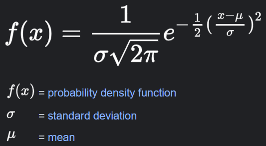
e=2.718... , pi = 3.14...
จุดเด่นของ normal distribution คือ มันจะมีรูปร่างเป็นระฆังคว่ำ
โดยมีค่าเฉลี่ย(μ)อยู่ตรงกลางเสมอ
‍
We say that X has a standard Normal distribution if µ = 0 and σ = 1

รูปเดิมใช้ซ้ำได้

●  probability function or probability mass function (PMF)

Distribution Functions(จะใช้ f เล็ก หรือ Pξ แล้ว CDFs จะใช้ F ใหญ่) with random variables ξ
ตัวอย่าง ที่เห็นชัดก็จะเป็นสูตร distribution function ของ Binomail ด้านบนที่เป็น discrete
แต่ Uniform distribution ด้านบนก็เป็น distribution function เหมือนกันแต่ไม่ได้เป็น discrete จึงเป็น PDF แทน
หากเรารู้ distribution function เราก็จะรู้ว่าค่า random variables แบบนี้ ความน่าจะเป็นที่เกิดขึ้นคือเท่าไร

PMF กับ PDF คือเครื่องมือชนิดเดียวกัน
PMF ใช้กับ discrete
PDF ใช้กับ continue

ตัวอย่างสำหรับ probability function ของ discrete random variables
‍
ยกตัวอย่างโยนเหรียญเหมือนเดิม จากการโยนเหรียญ 2 ครั้ง ติดกัน
หากได้หัว(H) เราจะให้ค่า = 1, แต่ถ้าได้ก้อย(T) เราจะให้ค่า = 0
ผลลัพธ์การโยนเหรียญที่ได้จะมี 4 กรณีคือ HH = 2 , HT = 1, TH = 1, TT = 0
ω = HH, HT, TH, TT
ξ(ω) = 2, 1, 1, 0
หากเอาตรงนี้มา plot ค่าความน่าจะเป็นของแต่ละเหตุการณ์เราจะได้

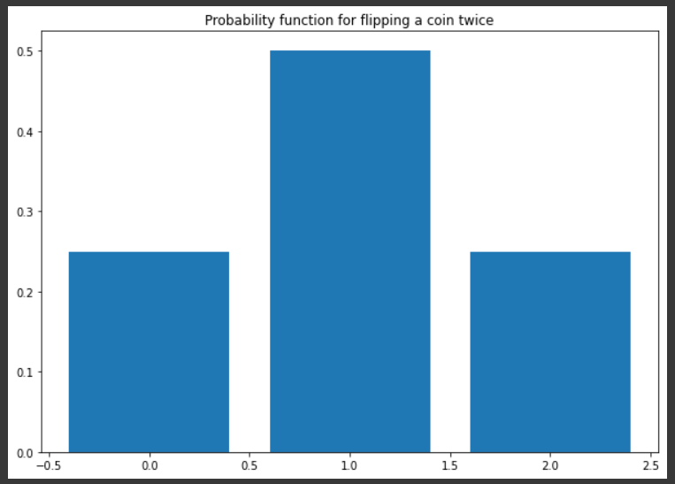
หรือถ้าเอามาเขียนในรูปแบบของ probability function

การแจกแจกเป็นแบบ Binomial ดังนั้นเราสามารถเอา distribution function ของ Binomial มาอธิบายได้

● Probability Density Functions (PDF)

จริง ๆ ก็คือ PMF ที่เอามาใช้วัดกับจำนวนที่เป็น continuous random variable

ถ้าเป็น continuous random variable
เราไม่สามารถที่จะเขียนแบบนี้ได้ เพราะ เราไม่รู้จุดเริ่มต้นมันที่ไหนและสิ้นสุดมันที่ไหน
0.00001 ? หรือ 0.000001 หรือ 0.0000001 หรือ 0.000000000000000000000000000000001 ?

เขียนแบบนี้ไม่ได้แล้วนะถ้าเป็น continued

ดังนั้นเราต้องเขียนแบบนี้แทน คือ 1/(b-a) โดยที่ a < b
example for Uniform [-1, 1] distribution

แล้ว CDF ของ Uniform [-1, 1] distribution ก็คือ
a = -1, b = 1

● cumulative distribution function (CDF)

เขาจะใช้ F ใหญ่
หมายถึง function ผลรวมของความน่าจะเป็น ตั้งแต่จุดเริ่มต้นถึงจุดที่เราสนใจ
โดยผลรวมของความน่าจะเป็นทั้งหมดรวมกันจะต้องได้ 1 เสมอ เหมือนเดิม

● properties of cumulative distribution function (CDF)

รูป CDF ของ Uniform distribution [-1, 1] จากด้านบน

Given a random variable X, we define the cumulative distribution function(or distribution function) as follows.

● Transformations of Random Variables

ถ้า X คือ random variable แล้ว f(X) คือ PDF และ F(X) คือ CDF

แล้ว Y = r(X)

โดย r() คือ function transformer จะเป็นอะไรก็ได้ เช่น x+1, 1/x, x^2

ตัวอย่าง

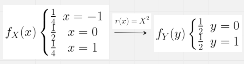
สิ่งที่เราเห็นจากการ tranform random variable จากด้านบนก็คือ
การ tranform random variable จะส่งผลต่อ PDF และ CDF

● Three Steps for Transformations

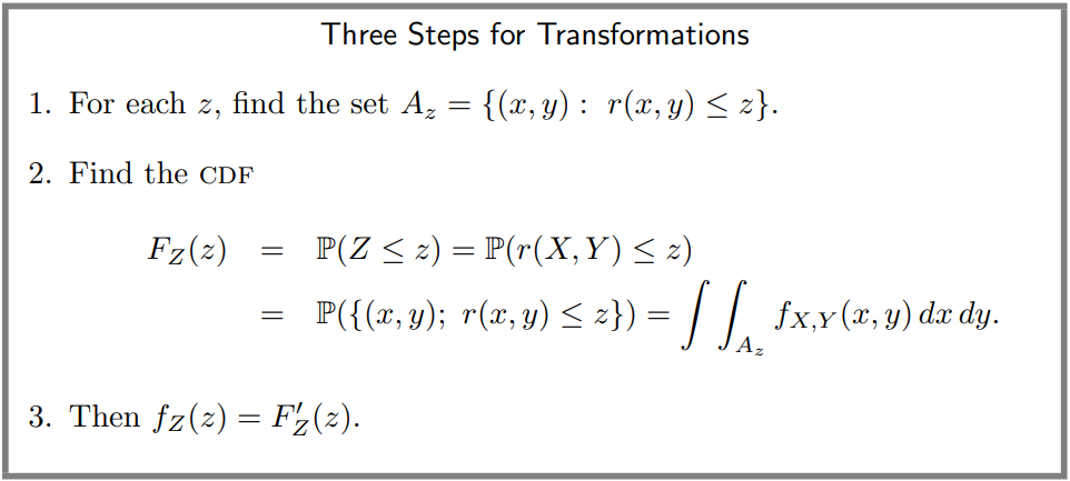
รูปจากหนังสือ All of Statistics: A Concise Course in Statistical InferenceBook by Larry A. WassermanBook preview

สิ่งที่น่าสนใจก็คือ ถ้าเราหา derivative ของ CDF ของ z เราก็จะได้ PDF ของ z

● Moment Statistics

In mathematics, a moment is a specific quantitative measure ofthe shape of a function.
Moments used to describe the characteristic of a distribution and shape of the data.

Suppose X is a random variable then
E(X) = first moment or Mean : measure of central tendency of a dataset.
E(X²) = second moment or Variance : measure of the spread or dispersion of a dataset.
E(X³) = third moment or Skewness : measure of the asymmetry of a dataset.
E(X⁴) = forth moment or Kurtosis : measure of the peakedness or flatness of a dataset.
...

ความตั้งใจที่เอามาใส่เพราะว่าอยากให้รู้ว่ามันคือค่า E(X) แต่ยกกำลังด้านในไปเรื่อย ๆ
ดังนั้นถ้าเราหา first moment ได้ ดังนั้นก็เราก็จะหา moment ในระดับที่สูงขึ้นไปได้
(x-mean)**2

● First moment : Expected Value, Mean, E(x), µ

E(X) = first moment or Mean : measure of central tendency of a dataset.
‍
วิธีการคิด

หรือถ้าเป็นวิธีที่คนปรกติคุ้นเคยก็คือ

● Expected Value of transformed variables

The Rule of the Lazy Statistician :
เพราะเรารู้อยู่แล้วว่า Y = r(X) ดังนั้นเราก็จะว่า PDF และ CDF ของ Y ก็มาจากของ X นั่นแหละ

ถ้าเราเจอตัวหนอนแล้วเราไม่เข้าใจ ก็ให้คิดว่ามันคือ Sum ในที่นี้คือ
ผลรวมของ r(x) นั่นก็คือค่า Y นั่นแหละ เอามาคูณกับ CDF ของค่า x นั้น

คือจริง ๆ E(X) = -1/4+0+1/4 = 0
E(X^2)=1/4+0+1/4=0.5

เรารู้ว่า E(Y) จากรู้ด้านขวา = 0.5
E(Y) = (1/2*0)+(1/2*1)=0.5

ดังนั้นคิดจาก E(X^2) ก็เท่ากันกับ E(Y) = E(0^2) = 0
ซึ่งข้อนี้เป็นกรณีพิเศษดังนั้นจึงคิดแบบ lazy ไม่ได้

● Second moment : Variance and Covariance

E(X²) = second moment or Variance : measure of the spread of a distribution or dispersion of a dataset.

● Properties of Variance

● Covariance and Correlation

Covariance and Correlation ต้องมาด้วยกันเสมอ

Covariance is a measure of the difference between two random variables X and Y.
It is denoted by Cov(X, Y) or σXY and is calculated using the following formula:

Covariance can be any value,
including negative values and it means X and Y tend to change in opposite directions.
A positive covariance indicates that X and Y tend to change in the same direction
A covariance of zero indicates that there is no linear relationship between X and Y.

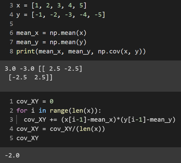
สิ่งที่น่าสนใจก็คือ ผมลองคิด COV(X, Y) จากสูตรด้านบน ในรูปได้คำตอบคือ -2.0
แต่ถ้าคิดโดย numpy จะได้ -2.5

ผมไม่คิดว่า numpy คิดผิด แต่ผมน่าจะคิดผิดเลยไป searh google ดู

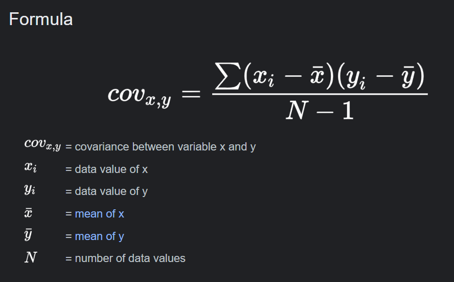
ถ้าหาค่า E(X, Y) เฉย ๆ เราก็จะหารด้านค่า N
ที่เวลาเราหา covariance แล้วหารด้วย N-1 เพราะว่า เป็นหลักการ "Bessel's correction"
ที่จะหาร sample variance และ sample standard deviation ด้วย N-1 แทน เพื่อลด bias
แต่การที่หารด้วย N-1 จะแลกมาด้วยค่า mean squared error ที่เพิ่มขึ้นแทน

● Covariance and Correlation

Correlation is a measure of the strength of "linear relationship"
and "linear direction" between two random variables X and Y.
It is denoted by Corr(X, Y) or ρXY

Corr(X, Y) = Cov(X, Y) / (σX * σY)

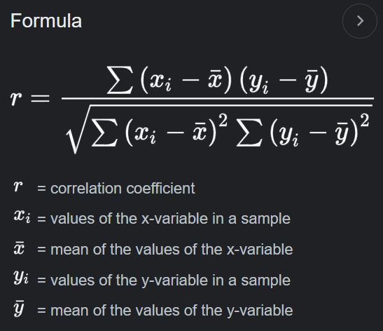
Correlation ranges from -1 to 1.

A correlation of 1 indicates a strong positive linear relationship between X and Y,
a correlation of -1 indicates a strong negative linear relationship,
and a correlation of 0 indicates no linear relationship.

Both covariance and correlation are used to describe the relationship between two random variables.
Covariance is a measure of the degree to which the variables vary together, while correlation is a measure of the strength and direction of the linear relationship between the variables. Both measures are useful for understanding the relationship between two variables, but correlation is often preferred because it is unitless and can be easily compared between different pairs of variables.

● Third moment : Skewness(ความเบ้)

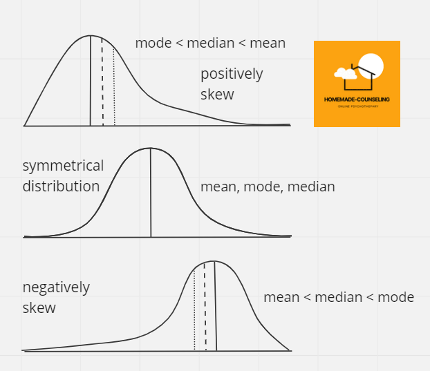
Skewness(γ) is a measure of the asymmetry of the probability distribution
of a real-valued random variable about its mean.

The skewness value can be positive, zero, negative, or undefined.

for γ between [-0.2, 0.2] the distribution can be assumed to be normal with respect toskew

● Fourth moment : Kurtosis(ความโด่ง)

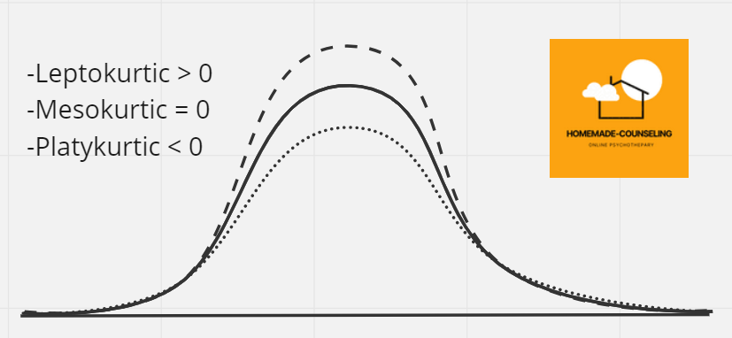
kurtosis from Greek kurtos, meaning “curved”.

Kurtosis is a measure of the"tailedness" of the probabilitydistribution of a real-valued random variable, i.e. its valuedescribes the thickness of the distribution’s tails.

If we would calculate the kurtosis of a normal distribution, we’d found that its value equals 3, no matter what parametersthe distribution has. A lot of mathematicians prefer to compare kurtosis of anydistribution with that of normal distribution. For that theysubtract three from the value of kurtosis.

For a normal distribution, the value of Kurtosis equals 3
If Kurtosis - 3= 0 : same peakedness as normal curve (Mesokurtic)

but if Kurtosis not equal to 3, there are the following cases:
Kurtosis - 3 > 0 : more peakedness than normal (Leptokurtic)
Kurtosis - 3 < 0 : flatter than normal curve (Platykurtic)
Kurtosis between 3 - 0.5 and 3 + 0.5] the curve can be considered normal with respect to kurtosis.

● Probability Inequalities

● Markov’s inequality

Markov's inequality is a result in probability and statistics that provides an "upper bound"
on the probability that a non-negative random variable exceeds a certain value.
‍
Using a bit of information about a distribution to learn something about probability of
"extreme events"

คือเรามีแต่ข้อมูล expected value แต่เราไม่มีข้อมูลอย่างอื่นเกี่ยวกับ distribution เลย
เป็นไปได้ไหมที่เราจะใช้ประโยชน์จากข้อมูลชุดนี้ได้

"if E(X) ≥ 0 and E(X) is small, then X is unlikely to be very large"

ยกตัวอย่าง expected value = 0.5
‍
ถ้า P(X≥0.5) ≤ 0.5/0.5 แล้วเราก็จะได้ว่า เราก็จะได้ P(X≥0.5) ≤ 1
แปลว่ามีโอกาส 100% ที่ X จะมากกว่า 0.5
‍
ถ้า P(X≥1) ≤ 0.5/1 แล้วเราก็จะได้ว่า เราก็จะได้ P(X≥1) ≤ 0.5
แปลว่ามีโอกาส 50% ที่ X จะมากกว่า 1
‍
ถ้า P(X≥10) ≤ 0.5/10 แล้วเราก็จะได้ว่า เราก็จะได้ P(X≥10) ≤ 0.05
แปลว่ามีโอกาสเพียง 5% เท่านั้นที่ X จะมากกว่า 10

ข้อดีก็คือถ้าเรารู้แค่ expected value เราก็สามารถใช้ Markov inequality ได้และ random variable ต้องไม่ติดลบด้วย
แต่ข้อเสียก็คือ มันก็ไม่ได้เที่ยงตรงมาก

● Chebyshev's inequality

Chebyshev's inequality provides a lower bound on the probability that a random variable is within a certain number of standard deviations of its mean. It states that for any random variable X with mean μ and standard deviation σ, the following inequality holds:

● Inequalities For Expectations

● Cauchy-Schwartz inequality

If X and Y have finitevariances then

● Jensen’s inequality

Examples of convex(shape V) functions are g(x) = x**2 and g(x) = e**x
Examples of concave(shape Λ) functions are g(x) = −x**2 and g(x) = log x.

● Convergence of Random Variables

หลักการของ convergence ที่ผมเข้าใจก็คือ ถ้าเพิ่มจำนวนของ random variable ขึ้นไปเรื่อย ๆ แล้ว
มันจะเข้าใกล้ค่าคงตัวค่าหนึ่งเสมอ

ยกตัวอย่างเช่น
กรณีที่ 1 : An ={1, 1, 1, 1, 1, 1, ...} ดังนั้น limit ของ 1 เมื่อ n → ∞ = 1
กรณีที่ 2 : An ={1/1, 1/2, 1/3, 1/4, 1/5, 1/6, ...} ดังนั้น limit ของ 1/n เมื่อ n → ∞ = 0
‍
แต่ประเด็นที่เราสนใจคือมันจะส่งผลต่ออะไรบ้าง เช่น moments 1, 2, 3, 4 , ค่าความน่าจะเป็น ก็ว่ากันไป
โดยและหนังสือบอกว่าเรื่องนี้เป็นแนวคิดที่สำคัญในสถิติ

โดย convergence จะแบ่งได้เป็น 2 ประเภทหลัก ๆ (มีมากกว่า 2 แน่นอน)คือ

**(ไม่รู้จะเอาไปไว้ตรงไหนดี) the law of large numbers (LLN) and the central limit theorem (CLT). The LLN basically states that the average of a large number of i.i.d. random variables converges to the expected value.

● converges in probability

ยกตัวอย่างเช่น เรารู้ว่าการโยนเต๋า 6 หน้า โอกาสเกิดของแต่ละหน้าจะเท่ากับ 1/6
ค่า expected value = 1/6(1)+1/6(2)+1/6(3)+1/6(4)+1/6(5)+1/6(6) = 3.5

ดังนั้นถ้าเราโยนเต๋าซ้ำไปเรื่อย ๆ โอกาสการเกิด 3 ก็จะเพิ่มขึ้นมากเรื่อย ๆ
และโอกาสของการเกิด 3 ก็จะเข้าใกล้ 1

ที่พูดมาก็คือ the law of large numbers (LLN) หมายถึงถ้าทำการทดลองไปเรื่อย random variable
จะเข้าใกล้ค่าใดค่าหนึ่งเสมอ

● converges in distribution

The central limit theorem (CLT) states that, under some conditions, the sum of a large number of random variables has an approximately normal distribution.

ถ้าทำการทดลองเยอะระดับหนึ่งมันก็จะกลายเป็น normal distribution เอง

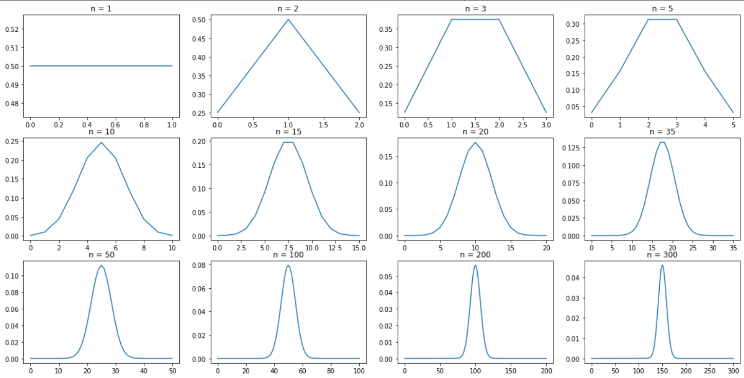
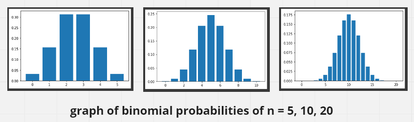
ตัวอย่างด้านบนเป็นการโยนเหรียญถ้าหัวจะนับเป็น 1 แล้วก้อยจะนับเป็น 0
แล้วรูปคือการแจกแจงของจำนวน n ครั้ง
เราจะเห็นได้ว่าถึงแม้ว่าค่าเฉลี่ยและการกระจายตัวจะแตกต่างกันออกไป
แต่สุดท้ายแล้วการแจกแจงก็จะรูปร่างใกล้ ๆ กับระฆังคว่ำหรือการแจกแจงปรกติครับ

● independent and identically distributed (i.i.d)

"IID" stands for "independent and identically distributed." It is a term used to describe a sequence of random variables that are independent of one another and have the same probability distribution.

Identically Distributed means that there are no overall trends–the distribution doesn’t fluctuate and all items in the sample are taken from the same probability distribution.

‍Independent means that the sample items are all independent events. In other words, they aren’t connected to each other in any wayIn other words, knowledge of the value of one variable gives no information about the value of the other and vice versa.

ตัวอย่างจากการทดลองโยนเต๋า 6 หน้าไม่ได้ถ่วงน้ำหนัก จากลูกเต๋าอันเดียวกัน
แต่เราก็รู้ว่าความน่าจะเป็นในการเกิดทุกหน้าคือ 1/6 เท่ากัน
แล้วเราจะโยนเต๋าเป็นจำนวน 100 ครั้ง

ซึ่งการโยนครั้งถัดไปไม่ได้มีความสัมพันธ์กับการโยนครั้งก่อนหน้าเลย
และเรารู้ว่าผลลัพธ์ทั้งหมดมาจาก distribution อันเดียวกัน นั่นคือ โอกาสเกิดทุกหน้า 1/6
ดังนั้นจึงเป็น i.i.d

● Likelihood

หลังจากเรารู้จัก PDF ไปแล้ว และ conditional probability ไปแล้ว
เรารู้จัก moment ที่ 1 และ moment ที่ 2 ไปแล้ว

P(x|θ)=L(θ|x)
‍

Likelihood and probability are two related but distinct concepts in probability and statistics.

Probability is a measure of the likelihood of an event occurring, expressed as a number between 0 and 1, with 0 representing an impossible event and 1 representing a certain event. For example, the probability of flipping a coin and getting heads is 0.5, because there is an equal chance of either outcome occurring.

Likelihood, on the other hand, is a measure of how likely it is that a particular hypothesis or model is true, given a set of data. In other words, it is a measure of how well a particular hypothesis or model fits the data. For example, if we have a model that predicts the outcome of a coin flip and we test it using a series of coin flips, we can measure the likelihood of the model being true by comparing the model's predictions to the actual outcomes.

In summary, probability is a measure of the likelihood of an event occurring, while likelihood is a measure of how well a particular hypothesis or model fits the data.

ทำไม่ต้องเปลี่ยนเป็น log? คำตอบคือ
เอาไปคำนวนและใช้ประโยชน์ได้ง่ายกว่า และได้คำตอบเดียวกัน

ยกตัวอย่างจากรูปที่เห็นด้านบน
เรารู้ว่าแต่ละการทดลองจะมีค่าเฉลี่ยและค่าส่วนเบี่ยงเบนมาตรฐานต่างกัน

ตัวอย่างเช่น n = 2 เราสนใจผลรวมที่ได้ 1
L(mean = 1 and std. =0.5 | ผลลัพธ์ของการโยนเหรียญรวมกันได้ 1) = 0.5 (ดูจากแกน y ในรูป)

ตัวอย่างจาก n = 3 เราสนใจผลรวมที่ได้ 1
L(mean = 1.5 and std. =0.75 | ผลลัพธ์ของการโยนเหรียญรวมกันได้ 1) = 0.375 (ดูจากแกน y ในรูป)

จากคนละโมเดลค่า likelihood ที่ 1 ก็จะแตกต่างกันออกไป
ถ้าผมเข้าใจไม่ผิดมันคือการวัดว่าโมเดลที่เรามีมันจะให้โอกาสเกิดเหตุการณ์ที่เราสนใจเป็นเท่าไรครับ

● Maximum Likelihood Estimation(MLE)

ถ้าเรามี distribution θ แล้ว distribution นั้นมีโอกาสเกิดเหตุการณ์ใดมากที่สุดหรือให้ค่า p เยอะที่สุด
ยกตัวอย่างเดิมจากรูปด้านบน

ถ้ากรณีที่ n = 2 โอกาสที่จะได้ 1 = 0.5 ซึ่งเยอะที่สุด นั่นคือ maximum likelihood

● ส่งท้าย